You must have seen some Excel spreadsheets with alternating colors in rows or columns. It can make the data more vibrant and easy to distinguish. Here I’ll introduce 2 commonly used methods to make a table like this.
How to Shade Every Other Row in Excel with Conditional Formatting
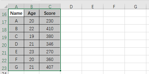
1. First, select the range of cells you want to shade.
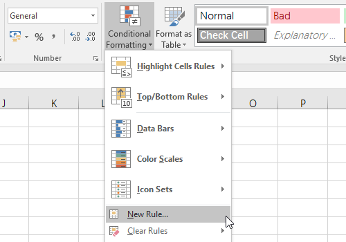
2. Switch to Home tab, click Conditional Formatting and choose New Rule… in the drop-down list.
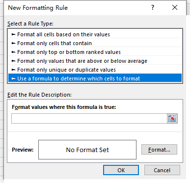
3. Select Use a formula to determine which cells to format as the rule type.
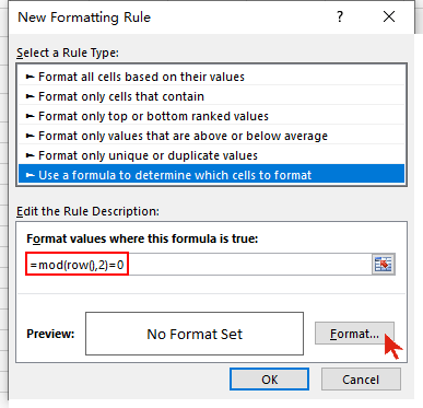
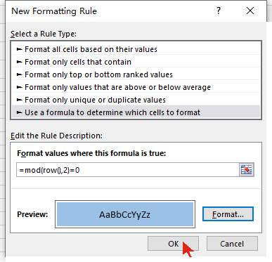
4. Enter the formula “=mod(row(),2)=0” in the textbox below Format values where this formula is true. Then click Format… on the lower right corner.
5. Choose a Background Color in Fill tab. Click OK to confirm it.
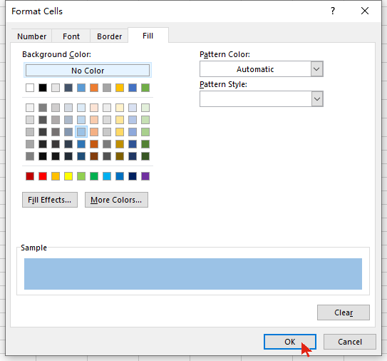
6. Hit OK again in New Formatting Rule window to implement the rule.
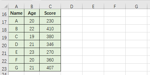
Now the rows of even number are shaded with blue. If you want to also apply colors to the rows of odd number, you can shade all the selected cells with a color at first and then follow above steps to apply another color to every other row.
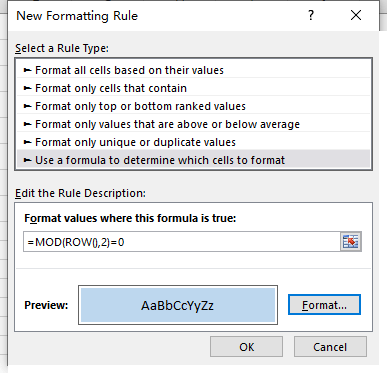
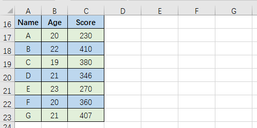
Or you can repeat the steps to add a new rule but change the formula into “=mod(row(),2)=1”

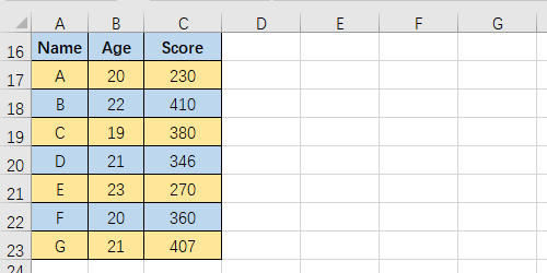
The color of odd number rows can be changed in this way as well.
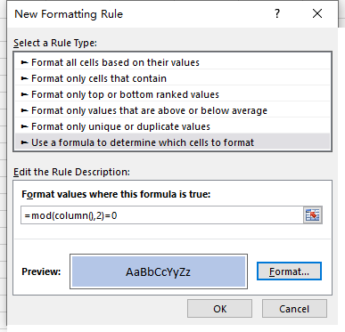
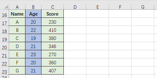
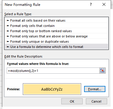
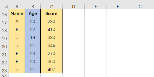
You can shade every other column in the similar way. Just change the formula a little bit to “=mod(column(),2)=0” and “=mod(column(),2)=1”
How to Apply Color to Alternate Rows and Columns with Table Style
If you are not good at remembering formula, try this method.
1. Select all the cells you want to shade.
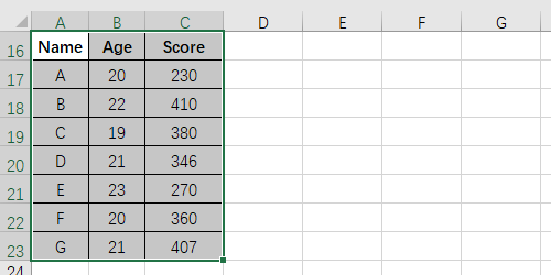
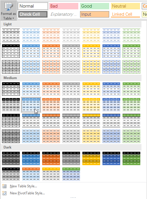
2. Switch to Home tab and click Format as Table in Style section to open the drop-down menu and choose a template you like.
3. Then choose a range of cells as the table area. Check or uncheck My table has headers according to your actual situation.
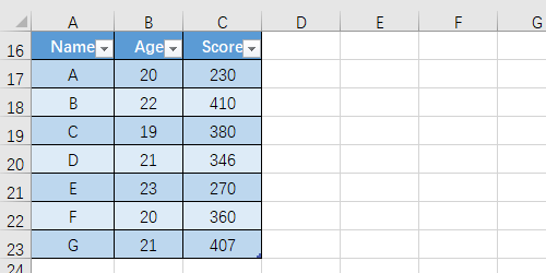
4. You can also adjust the color and apply some options to the table in the Table Tools of Design tab.

But if you want to apply colors to alternating rows or columns more freely, you’d better try the first method using Conditional Formatting.

Leave a Reply