25 Microsoft Excel Tips for Beginners Who Work at Office

For an office worker, it’s very important to grasp some commonly used Excel skills to process the data in a spreadsheet. Only in this way they can save the time to do more constructive work and improve themselves. So, how to use Microsoft Excel smartly to boost the working efficiency?

In this post I collected some useful tips about Excel features and functions as a reference. If you are one of those office workers who want to do better in processing data, and using less time. I’m sure you can benefit from these tips.

1. The Interface of Excel 2019

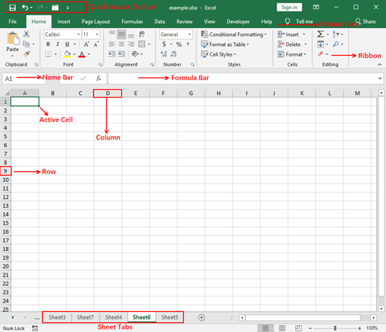
This tutorial is based on Microsoft Excel 2019. You can see the basic elements of its user interface below.

2. Insert Multiple Row or Columns in Excel

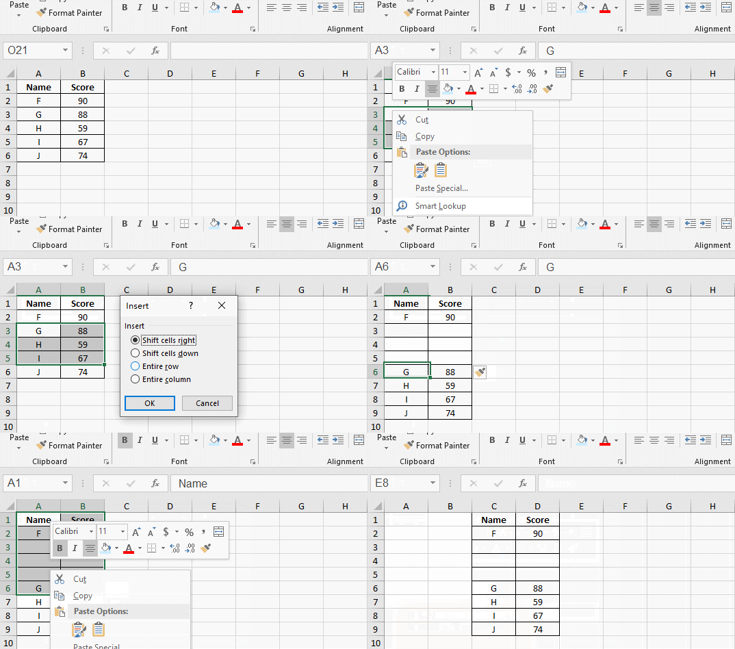
You probably know how to add a new row or new column in Excel spreadsheet, but if you need to insert multiple rows or columns, repeating this operation can’t be the best idea.

You can drag the mouse to select multiple rows (or columns) at first, then right-click the selected area and click Insert in the menu. The number of rows inserted will be equal to the number of rows you selected.

3. Merge and Split Cells in Excel

A spreadsheet can’t be done without any adjustments and modifications. It’s also common to merge multiple cells or split the content in one cell.

You may already know there’s a merge button in the Home tab of Excel. But if you use it to merge 2 cells with different texts, the merged cell will only keep the upper-left value and discards other values.

To merge multiple cells and keep all the contents of them, there are 2 functions you can try:

Create a new column and Enter the formula: =A2&B2 to merge the contents in A2 and B2.

If you want to add a space between the contents of A2 and B2, just enter: =A2&“ ”&B2.

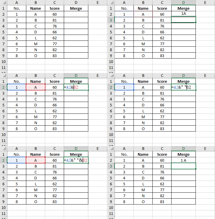
Or, you can also use this formula: =CONCATENATE(A2,B2).

To split the content from one cell to multiple cells, or from one column to multiple columns, you can select the cells you want to split, and try using Text to Columns in Data tab.

And if there are no symbols like commas or tabs separating each field, choose Fixed width to continue and create break lines by yourself.

Then specify the Destination to output the data.

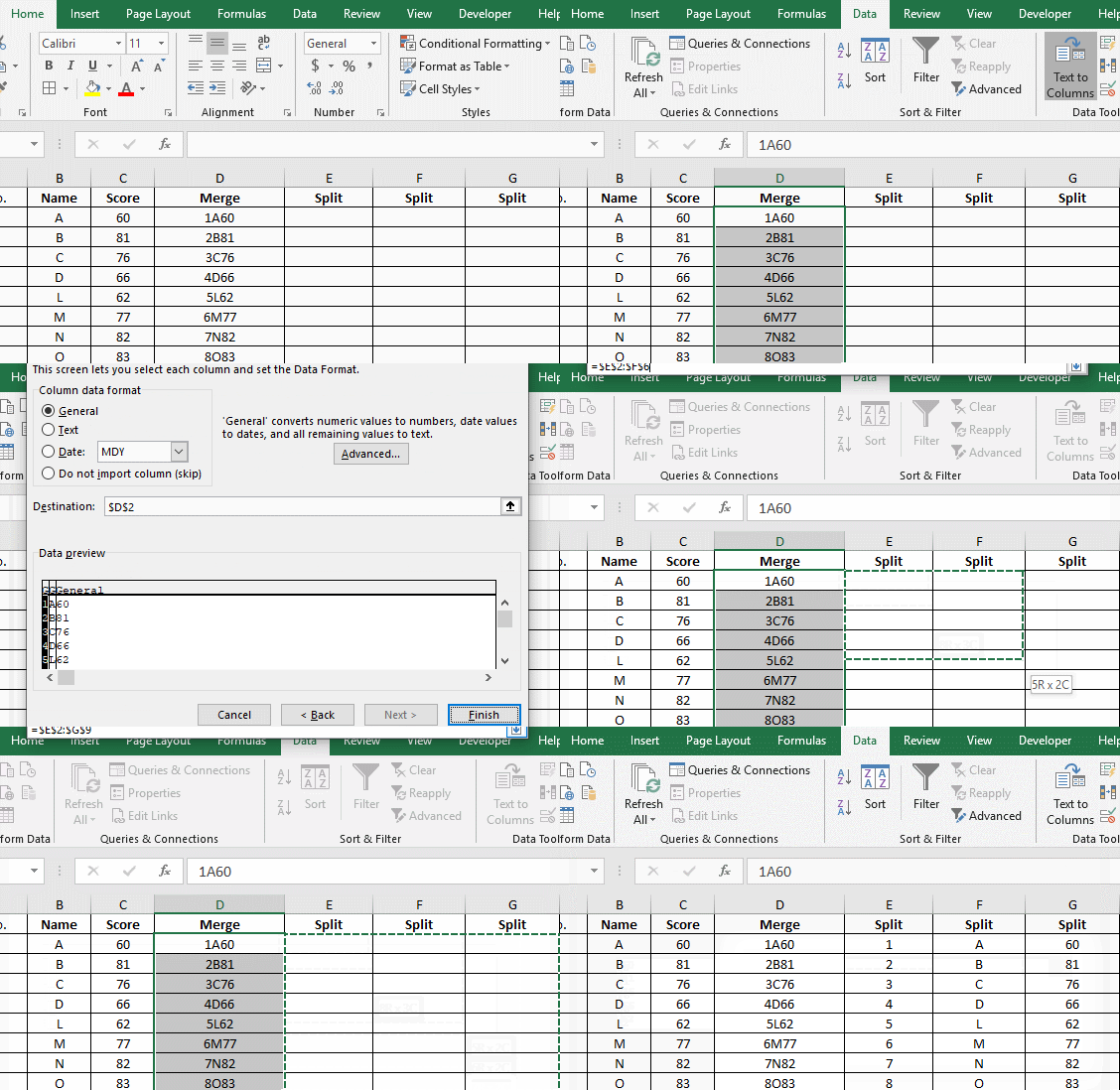
You can try another quick way to split data using Flash Fill.

4. Replace Specific Content in All the Worksheets

You must often create multiple sheets in an Excel file to process different but related data, and sometimes you may need to replace a specific word or value in all the sheets to ensure their correctness and consistency.

Instead of adjust each sheet separately, you can use a simple trick to boost the efficiency.

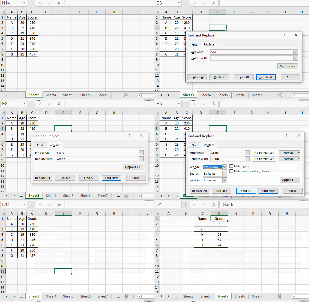
Press [Ctrl+H] in any of the sheets to open Find and Replace window. Input the text you want to find and the text you want to replace with.

Hit Options button on the lower right. Then click the small down-arrow beside Within Sheet and choose Workbook instead. Thus the change will be applied to all the sheets in the workbook.

5. Undo or Redo Your Last Action in Excel

There are always some faulty operations when dealing with complicated tables and sophisticated data in Excel. If you don’t know exactly what the spreadsheet looks like a second before, how can you recover it to the correct version?

In fact, you can simply undo your last action or multiple actions before by pressing [Ctrl+Z].

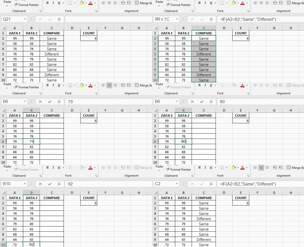
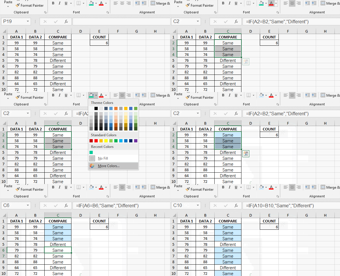
On the contrary, if you want to apply an action to multiple discontinuous cells or even cells in different spreadsheets, you can make use of [F4] to redo your last action.

6. Let Excel Do the Repeated Calculations for You

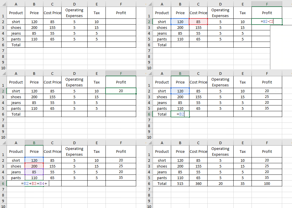
To deal with a huge amount of data in Excel worksheets, you don’t need to do all the calculations by yourself or with a calculator. There’re some formulas can help you processing data quickly and also easy to use. You don’t even need to remember them specially.

To calculate the summation of several values, you just enter =value 1+value 2+value 3 in the cell and press [Enter] to work it out.

To do subtractions, you can enter =value 1-value 2-value 3.

Moreover, you can combine summations and subtractions in a formula.

And don’t forget to place the cursor at the bottom-right corner of the cell and drag it (which is so called fill handle) to apply the same formula to multiple cells. In this way you can do calculations in a batch of cells at once.

7. Display all the formulas in Excel Worksheet

When a colleague sends you his or her worksheet, you may find it contains a lot of functions.

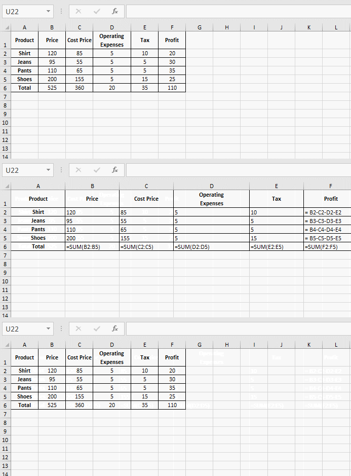
Want to know what formulas your colleague uses? It’s OK to click the cells one by one. But if you think it’s too much trouble, try using the shortcuts [Ctrl+~] to display all the formulas.

It can quickly display all the used formulas. Similarly, you can press [Ctrl+~] again to hide them.

8. Make Adjustments to Multiple Sheets in Batch

What if there are several worksheets with the same content and you want to make the same changes to them all?

It’s an easy trick:

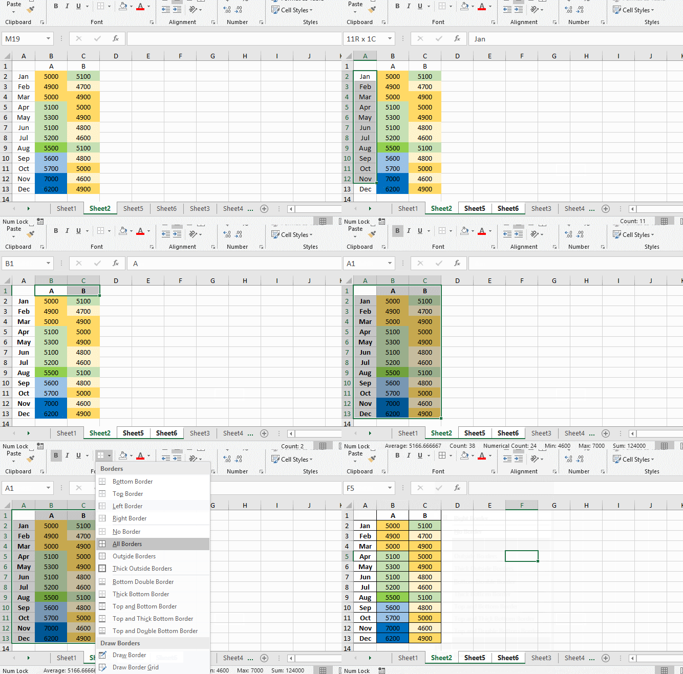
press and hold the [Ctrl] key while clicking the sheet tabs in Excel.

Then whatever you do to one of these sheets, the changes will be applied to all the selected sheets at the same time.

9. Use Clipboard to Merge the Data from Different Tables

Each department has sent a table and you want to put them together, is there a way to merge all the data at once? In fact, you can use clipboard to merge tables quickly instead of cut & paste separately.

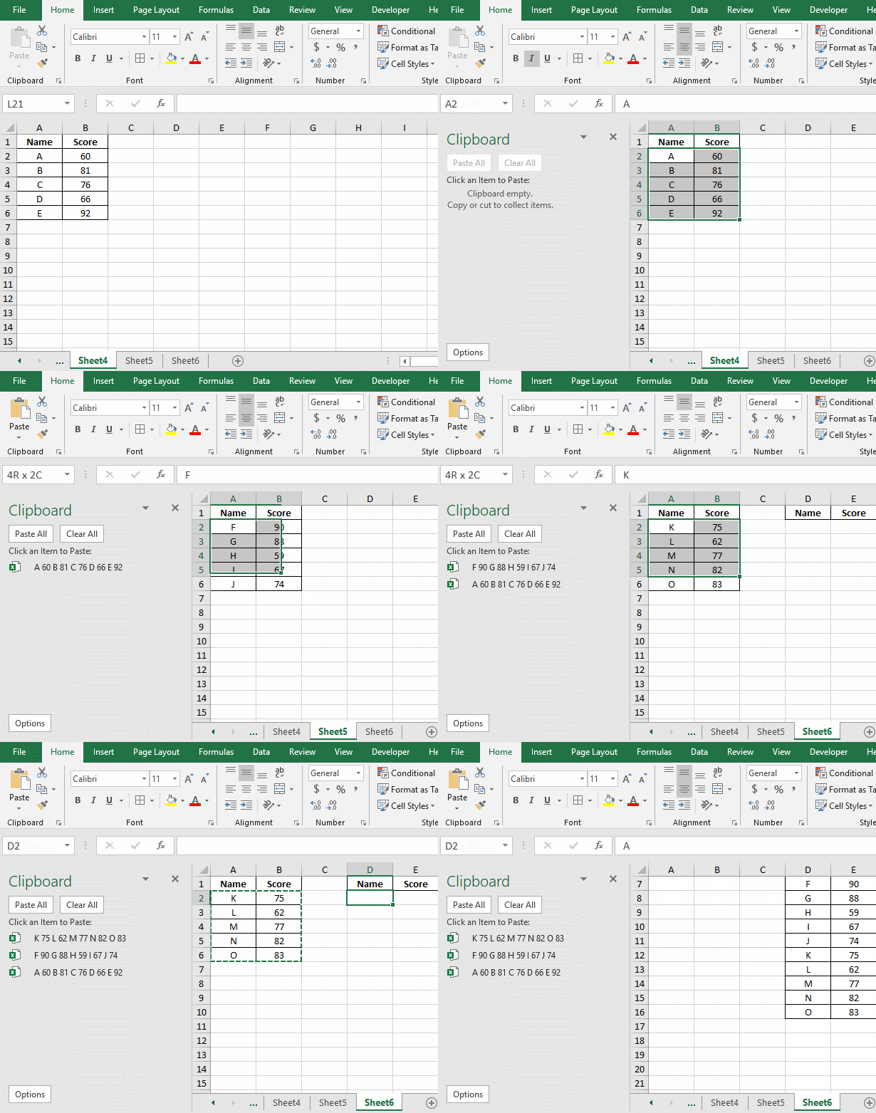
Click the small arrow at the bottom-right corner of Clipboard section in Home tab to open the Clipboard.

Then select the range of cells you want to merge and click Copy button separately.

Click Paste All on Clipboard to merge all the selected data at last.

10. Add Commands to Quick Access toolbar

If there some features of Excel you use frequently but not included in the quick access toolbar by default, you can add commands to quick access toolbar manually to use them more conveniently in the future.

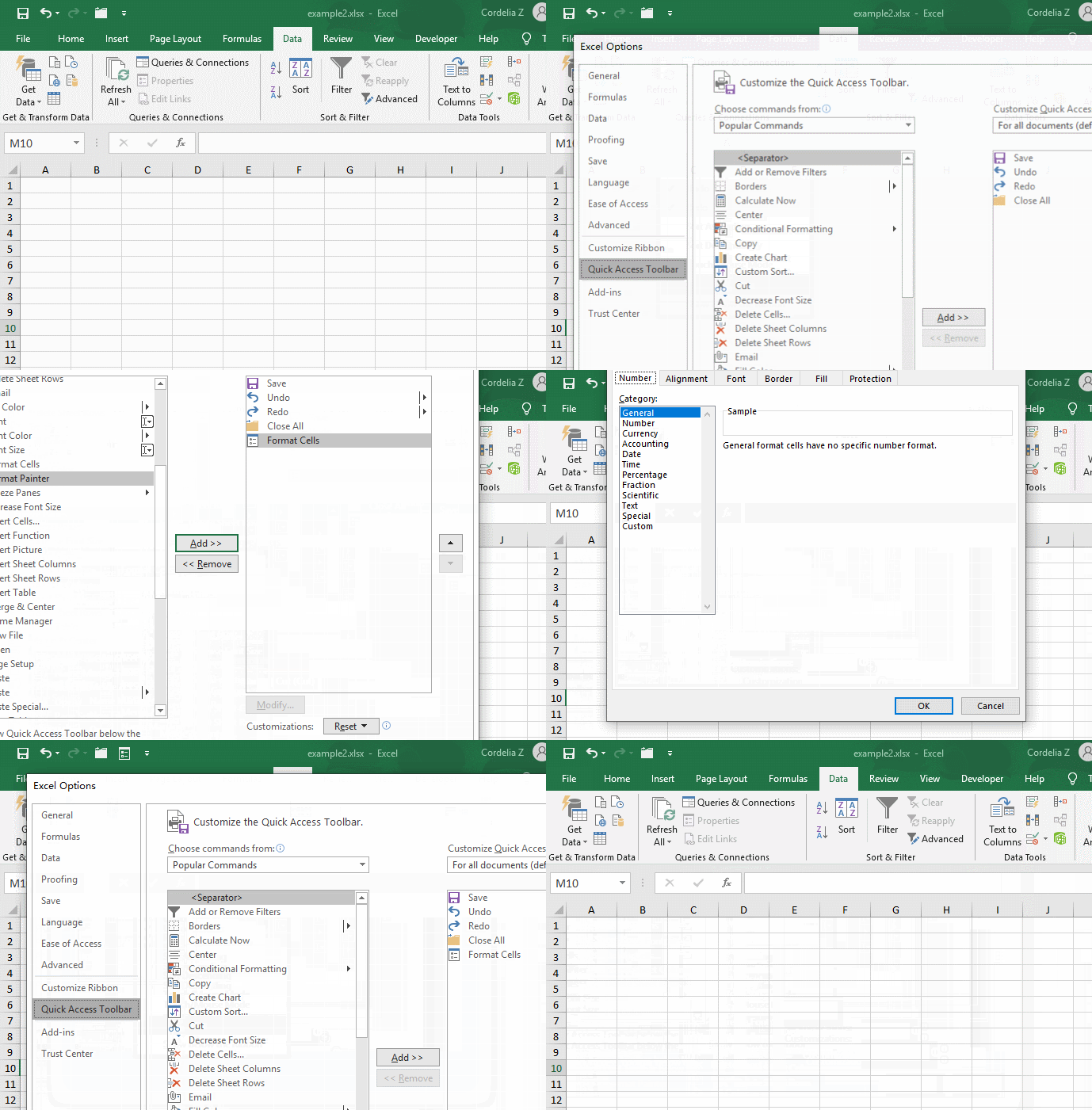
Just click the small arrow on the quick access toolbar and select More Commands… in the menu.

Then choose the commands to add them in the Quick Access Toolbar panel in Excel Options, and hit OK to confirm it.

Next time you can find the feature directly in quick access toolbar. If you want to delete it, just repeat the process and Remove it from the list in Quick Access Toolbar.

11. Apply Color to Specific Cells Using Conditional Formatting

Conditional Formatting can change the format of specific data according to the conditions you set.

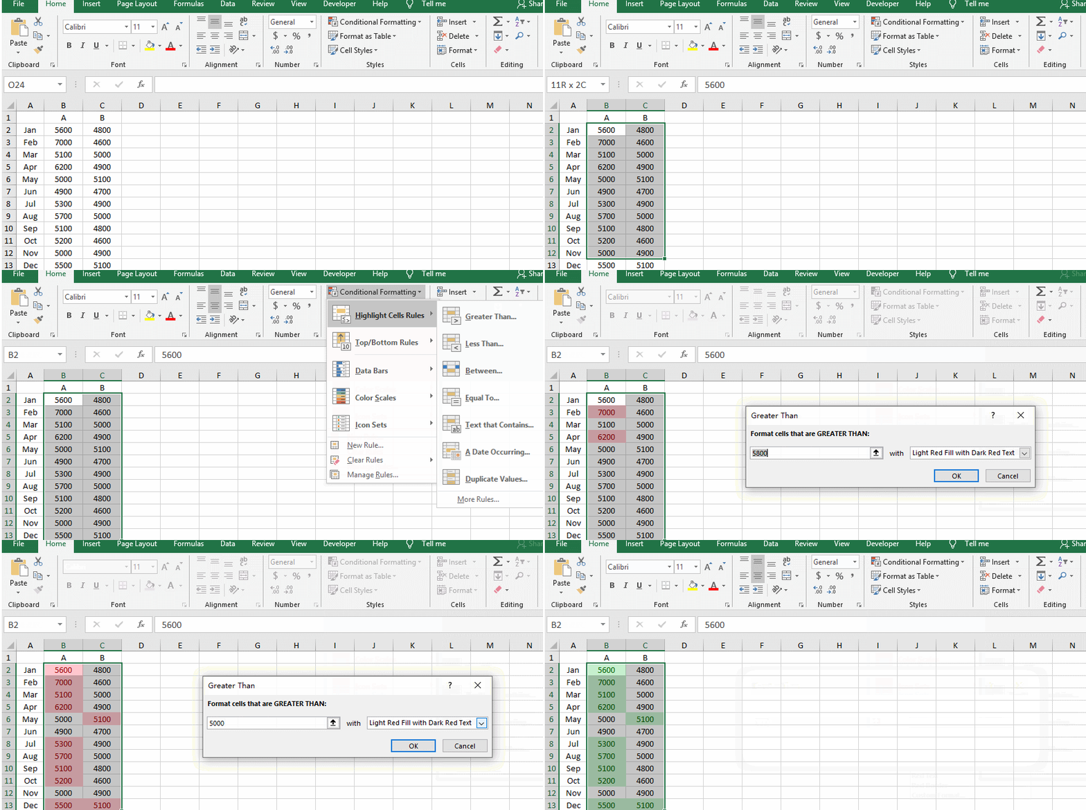
For example, if you want to highlight all the data greater than a fixed amount in a spreadsheet, you can use Conditional Formatting to shade them in batch.

Just select the range of cells you want to apply the conditional format, then click Conditional Formatting in Home tab.

There are many existing rules in the drop-down list you can directly choose and use.

In my case, I want to shade all the data larger than 5000 in column B and column C. So choose Greater Than… in Highlight Cell Rules. Type the number 5000 and choose a format color in the popping out window.

12. Sort the Data by Color in Microsoft Excel

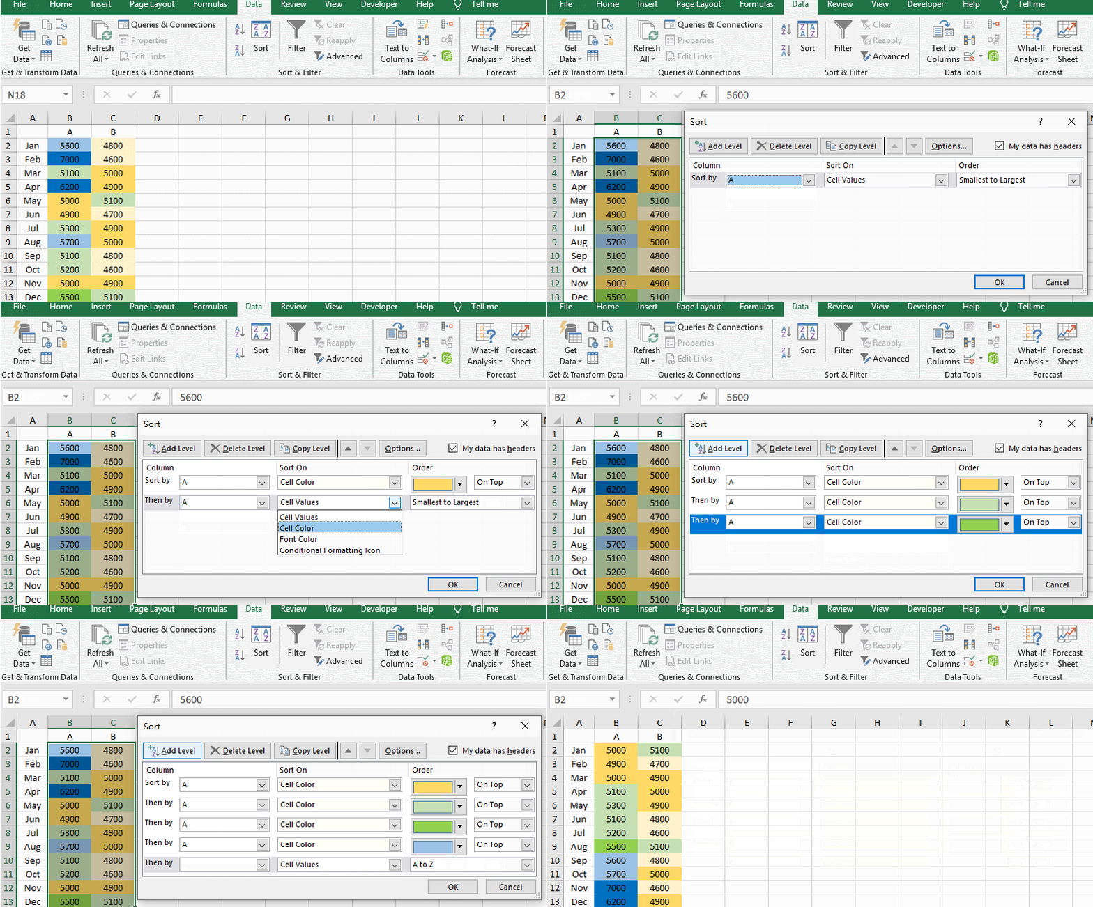
While editing a spreadsheet in Excel, you might need to change the color of some text or cells to make them more readable. And in some cases, like analyzing the data of monthly sales or wages, you can sort the data by color in Excel.

Go to Data tab and click Sort in Sort & Filter group.

Choose the column you want to sort in Sort by and select Font Color or Cell Color in Sort on.

Choose the color and set its Order. If there are multiple colors in the column, you can Add Level to create more rules. Click OK after all the settings.

13. Filter the Data by Cell’s Color in Excel

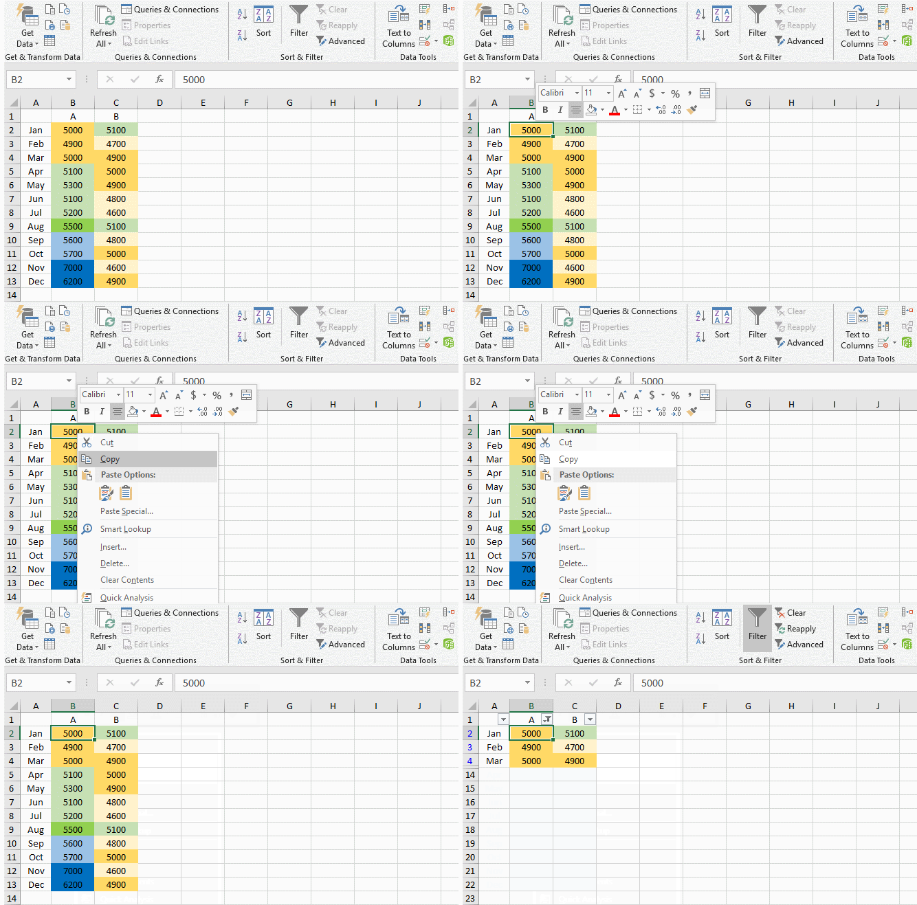
Similarly, sometimes you may also need to single out the cells with specified color.

Just right-click the color you want to screen out, and select Filter – Filter by Selected Cell’s Color in the menu.

14. Make Images Aligned to Gridlines in Excel

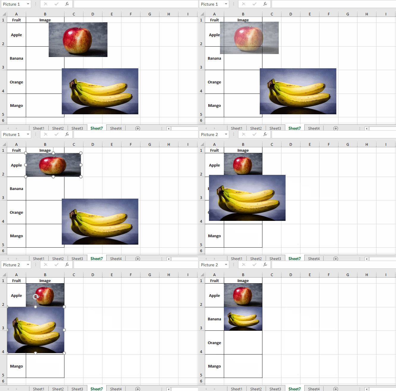
When you make a spreadsheet with pictures in Excel, you might spend much time on resizing the picture to fit in the cell.

To save your time and effort, you can press and hold the [Alt] key while dragging the 4 boundaries of the picture to resize it.

You’ll find the picture is easily aligned to the gridlines of the cell, which is much more convenient.

15. Insert Mini Charts (Sparklines) in Excel Cells

The mini charts, also known as sparklines, can display the trends of data in small cells. They are more informative than pure text and number, but with the smaller size than ordinary charts.

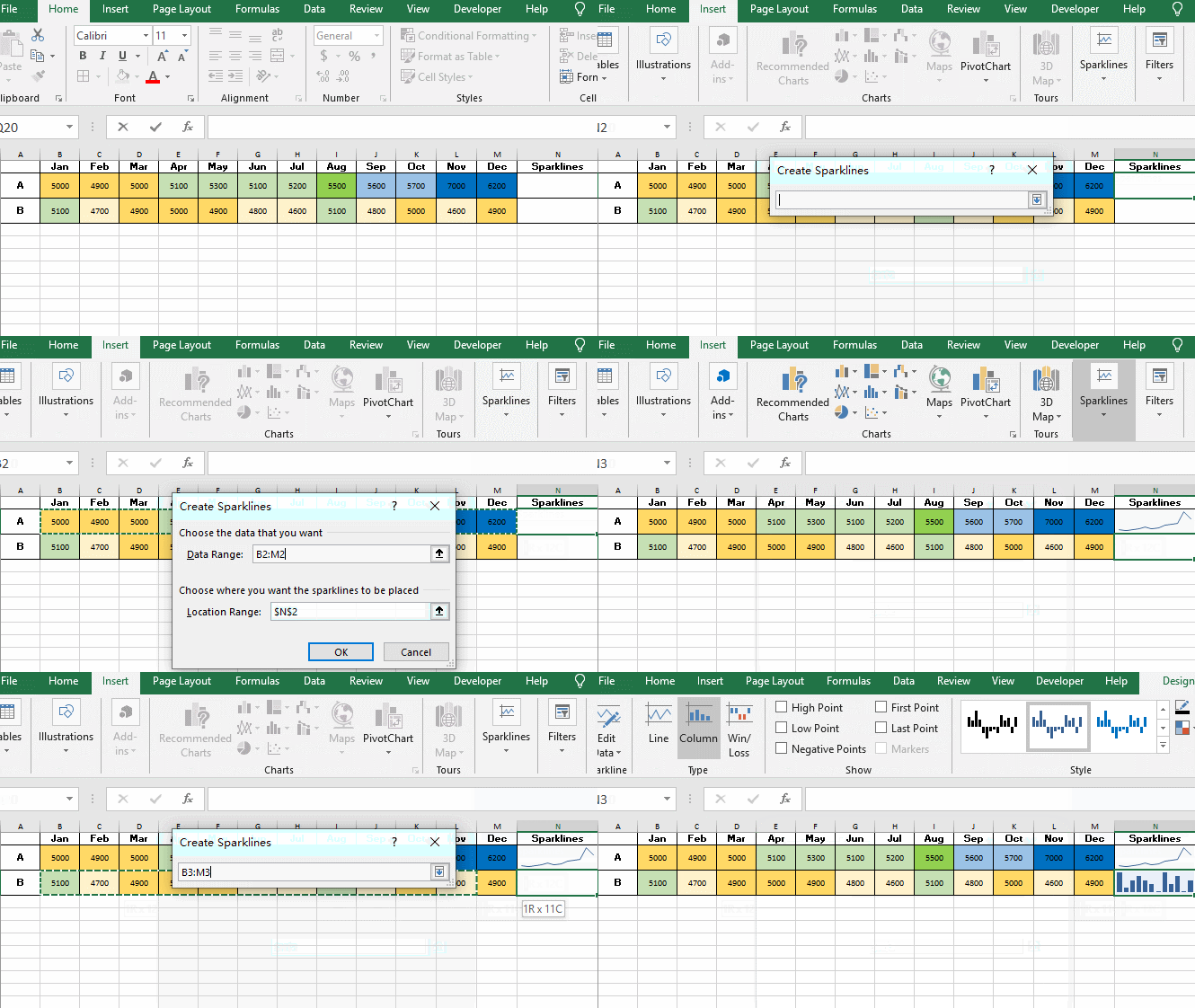
To insert a sparkline in an Excel cell, just click the cell and switch to Insert tab.

Choose a type in Sparklines section, then specify the range of cells as the data source.

The sparklines can be created immediately.

16. Quick Access to Drop-down Menu

While filling in some repeated contents, such as gender, name and so on, you can create a drop-down list to save the time of typing the same text.

But do you know with the shortcuts [Alt+↓], you can get the similar result without a drop-down list?

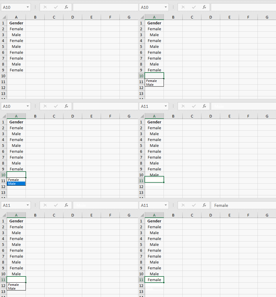
After typing some texts in the column, you can click the next cell and press [Alt+↓] on your keyboard.

It enables you to select an option from the existing texts and fill it in the current cell.

17. Create an Uninterrupted Sequence in Excel Column

After filling a list of sequence numbers in Excel, you may find some of the data are redundant and need to be removed.

But if you delete them directly, some of the sequence numbers will be missing. You must to fill up them manually, which is too much trouble.

Here, I’ll show you a function to create an uninterrupted sequence in Excel.

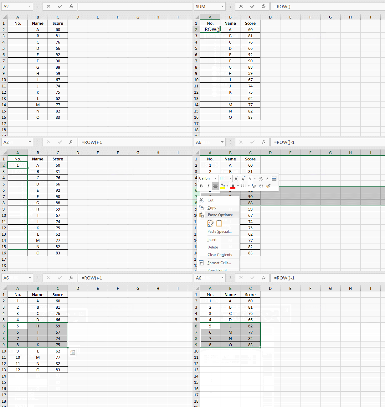
You just need to enter the formula: =ROW()-1 in the first cell, and drag your mouse to use fill handle filling the whole column automatically.

The sequence created in this way will always be uninterrupted even if you delete some rows in the spreadsheet.

18. Compare the Data in Two Columns

If you got 2 columns of similar data in Excel and want to compare them, it’s apparently not the best idea to find the difference row after row by naked eyes.

With Excel functions, you can compare the two columns of data using a single formula.

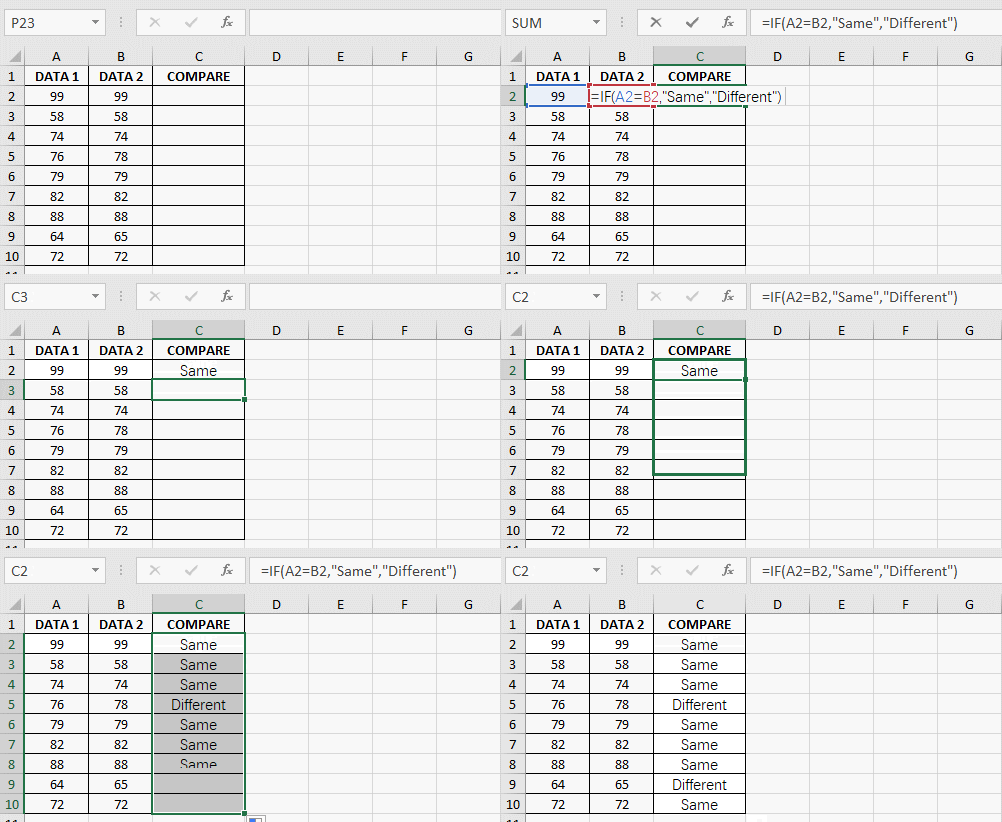
Create a column beside the 2 columns, then enter the formula: =IF(A2=B2,”Same”,”Different”) in the cell C2.

It means if the data in A2 and B2 are all the same, the text “Same” will be displayed in C2. Otherwise it will show “Different”.

After that, apply this formula to all the cells that beside the data you want to compare.

19. Count the Repetitions in Excel

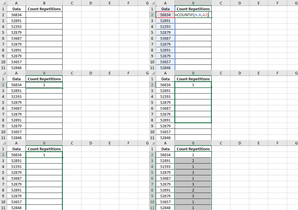
If a data appears in an Excel column for multiple times, and you want to figure out how many times exactly it’s repeated, the COUNTIF function can help you to count the repetitions.

Create a column beside the list of data.

Enter =COUNTIF(A:A,A1) in B2, it will check all the data in column A and show how many times the data in A1 repeated.

20. Remove the Duplicates Lines in Excel

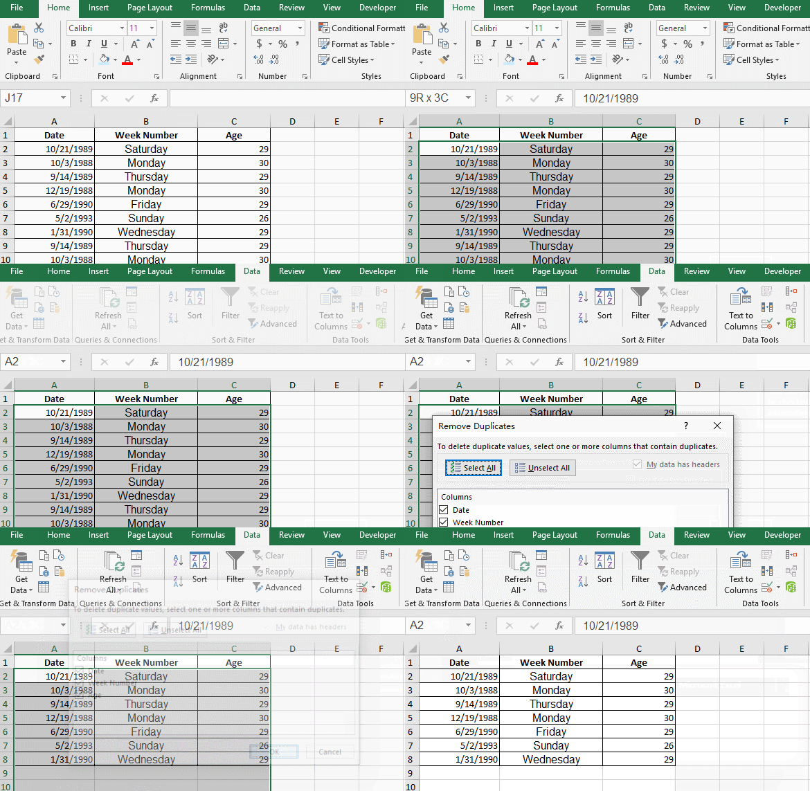
In addition to find duplicates in a spreadsheet, you may also need to remove the duplicate lines to simplify the content. Luckily Excel has a function to solve this problem directly.

First, select all the cells you want to remove duplicates from. Go to Home tab, click Remove Duplicates in Data Tools section.

Then select all the columns that may contain duplicates in the popping out window. Hit OK to implement it. All the duplicate lines in the selected area will be removed right away.

21. Count the Data that Meet the Specific Criteria

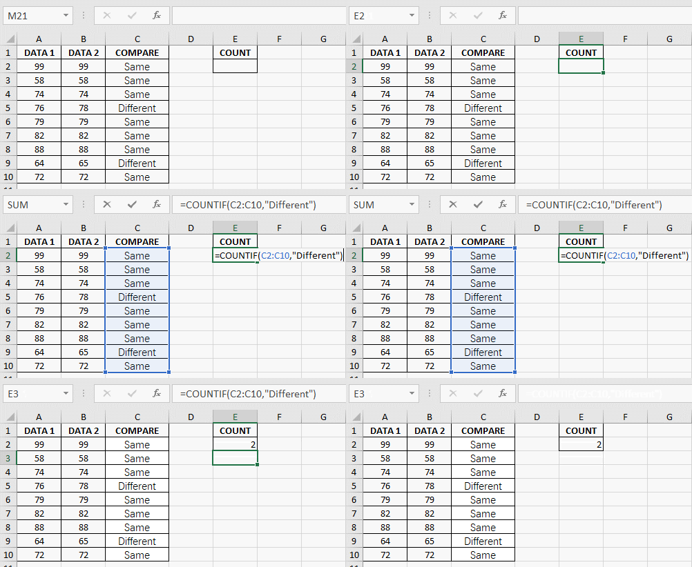
In an Excel spreadsheet containing so much data, how can you count the cells that meet the specific criteria?

Excel functions can help you to get the results with a simple formula: =COUNTIF(range,criteria)

For example, to count all the cells with the text “Different” in column C, you can enter the formula in a blank cell: =COUNTIF(C2:C10,“Different”), then press [Enter] to get the result.

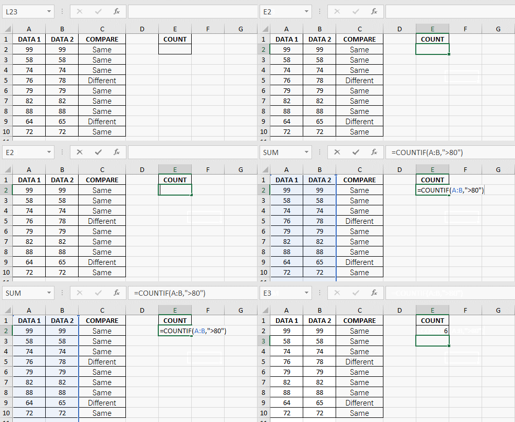
Similarly, if you want to count all the data greater than a specific number in column A and column B, the formula can be like: =COUNTIF(A:B,”>80″).

22. Fully Display Numbers in Excel Cells

Due to scientific notation, the long numbers (more than 11 digits) inserted to Excel cells will be abbreviated by default.

So how can you fully display long numbers in Excel?

One thing you can do is changing the format of these cells.

Right-click them, choose Format Cells and selecting Text in the Category before entering long numbers.

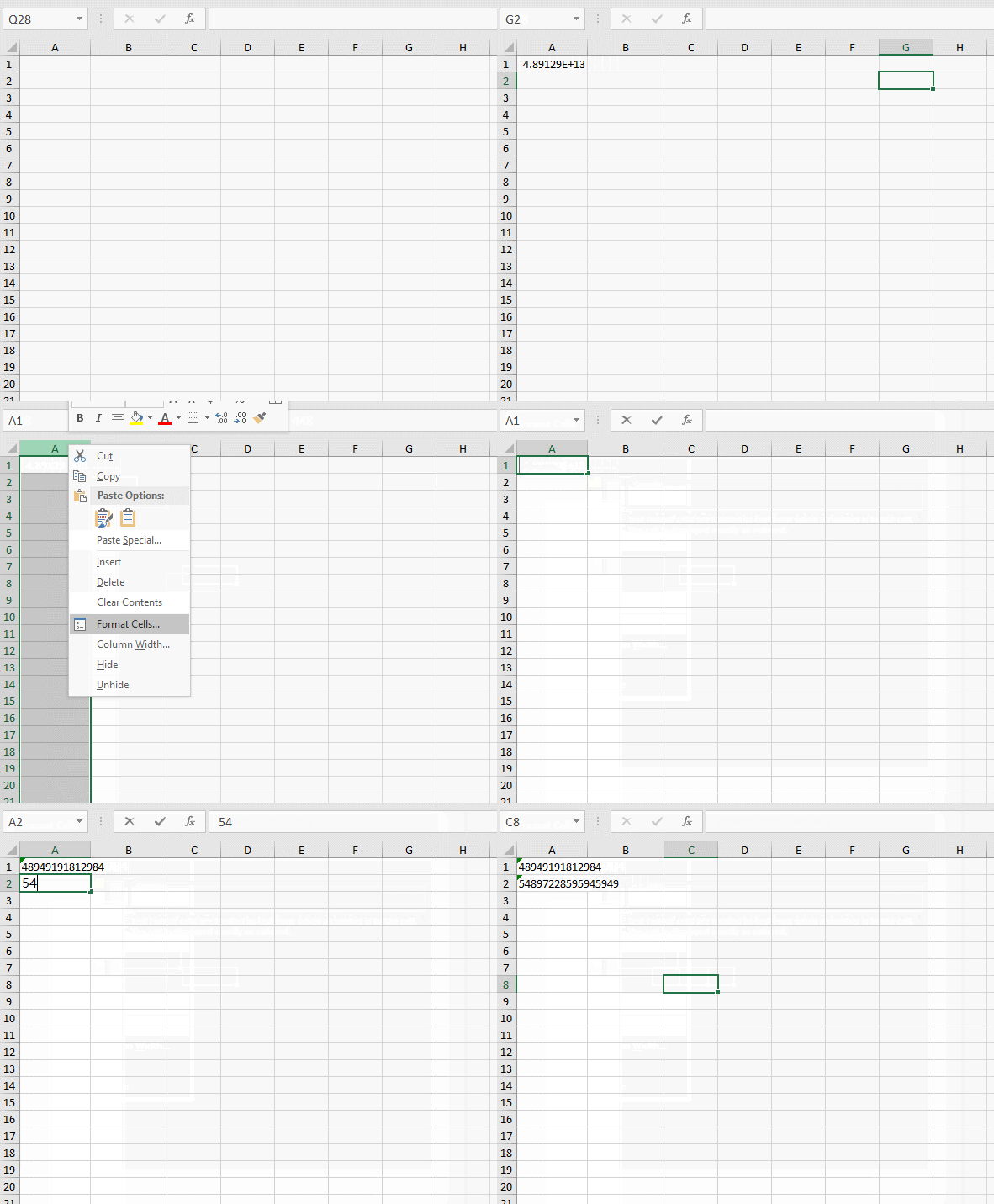
And if you want the long numbers to be displayed as phone numbers, you can change it in Format Cells as well. Check the detailed steps to display numbers as phone numbers.

23. Calculate the Week Numbers According to the Dates

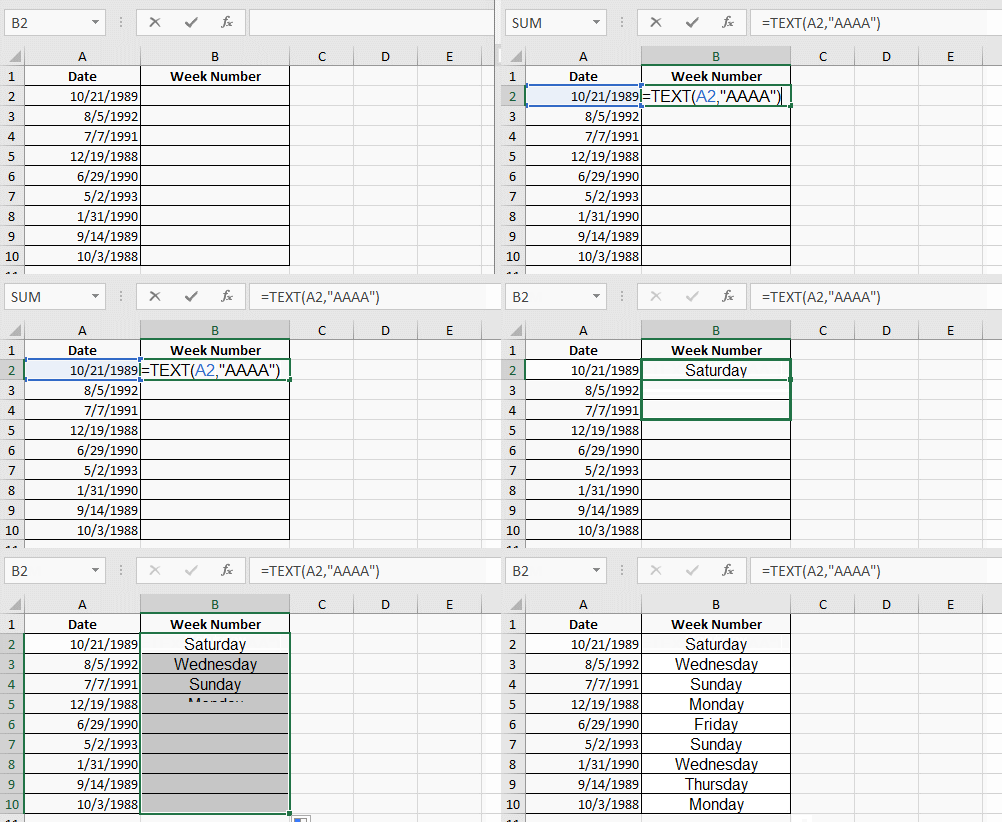
If the data of date has been collected in an Excel spreadsheet, and you want to know what day of the week it is, is there any way other than looking at your own calendar?

As you know, Excel functions are very powerful, there’s almost always a proper formula for solving your problems in Excel. It’s no exception in this case.

Create new column to output the week numbers beside the column of dates.

In my case the first cell of date is A2, so enter the formula: =TEXT(A2,”AAAA”).

Then press [Enter] to work it out and apply the formula to all the cells in the new column.

24. Calculate the Ages According to the Birth Dates

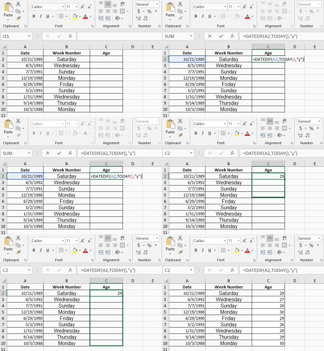
If you are a HR who wants to record the ages of all the employees, and the only data you have are the birthdates of them, you can of course figure out their ages by your own.

But if there are so much data that you can’t process all manually, is it possible to calculate their ages using functions automatically?

To save your precious time on this problem, there’s a powerful formula you should know.

Create a new column called “Ages” and input =DATEDIF(A2,TODAY(),”y”) in C2.

You can then see their ages after hitting [Enter] key and applying this formula to all cells in column C.

25. Protect Excel Files with Password

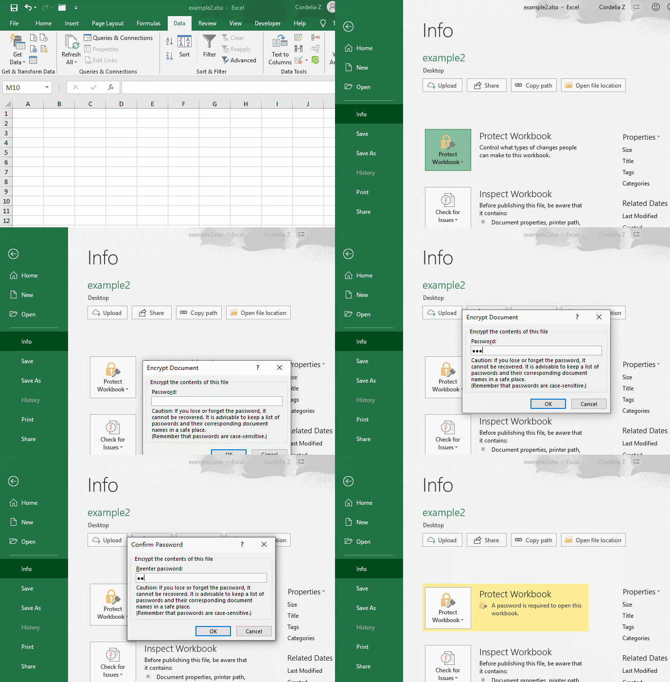
An Excel spreadsheet might contain some important information that you don’t want others to view. To prevent it from being peeked or even tampered, you can set a password to your Excel files.

Go to File tab and click Protect Workbook in Info panel.

Select Encrypt with Password, enter a password in the popping out window.

Re-enter it and click OK to confirm the setting. Then you document is protected. Next time you must enter the right password to open it.

26. Conclusion

With these tips for Microsoft Excel, you’ll be sure to processing data better and quicker at work. There are so much more useful tips to learn, of course, as Excel is such a powerful tool. For example, you can find specific data in Excel using VLOOKUP function, get corresponding result according to specific criteria by IF function, using shortcuts in Excel to boost your work efficiency, etc.

It’s not as difficult as it looks to use Excel. With these skills, you can do much more better in data arrangement and save your time to do more creative work.