
Microsoft Excel is a widely used office software which you must have tried or at least heard in life. It’s convenient, powerful and also complicated for some newbies since there seems to be too much to learn. They may end up doing repetitive work manually without knowing how to use Excel formulas to complete their tasks. It’s undoubtedly a huge waste of time and effort.
In fact, you don’t need to spend much time on learning all the things about it. There are some useful Excel functions can greatly improve your working efficiency, and best of all, they are all easy to master.
1. SUM Fuction
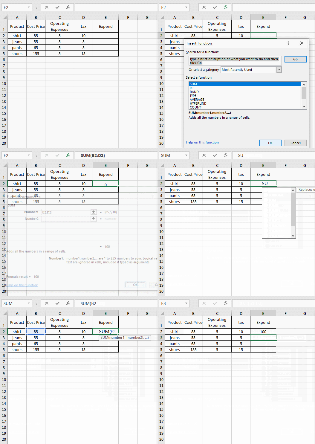
Comparing to calculate the total amount of a lot of data manually, Excel itself can do a better and quicker job to calculate the summation. It’s called SUM function. To make use of it:
① Select the cell you want to output the result of calculation, then click the icon of Insert Function above the table.
② Choose SUM in the popping out window and hit OK.
③ The formula will be filled in the cell and a window called Function Arguments will pop out. You can click the up arrow to select the range of data to calculate or type it manually. In my case I want to sum the data from B2 to D2 (including C2), so the complete formula should be “=SUM(B2:D2)”.
④ If you want to sum the data of B2 and D2, you should set the value of Number 1 and Number 2 as B2 and D2 separately, or input complete the formula as “=SUM(B2, D2)” directly.
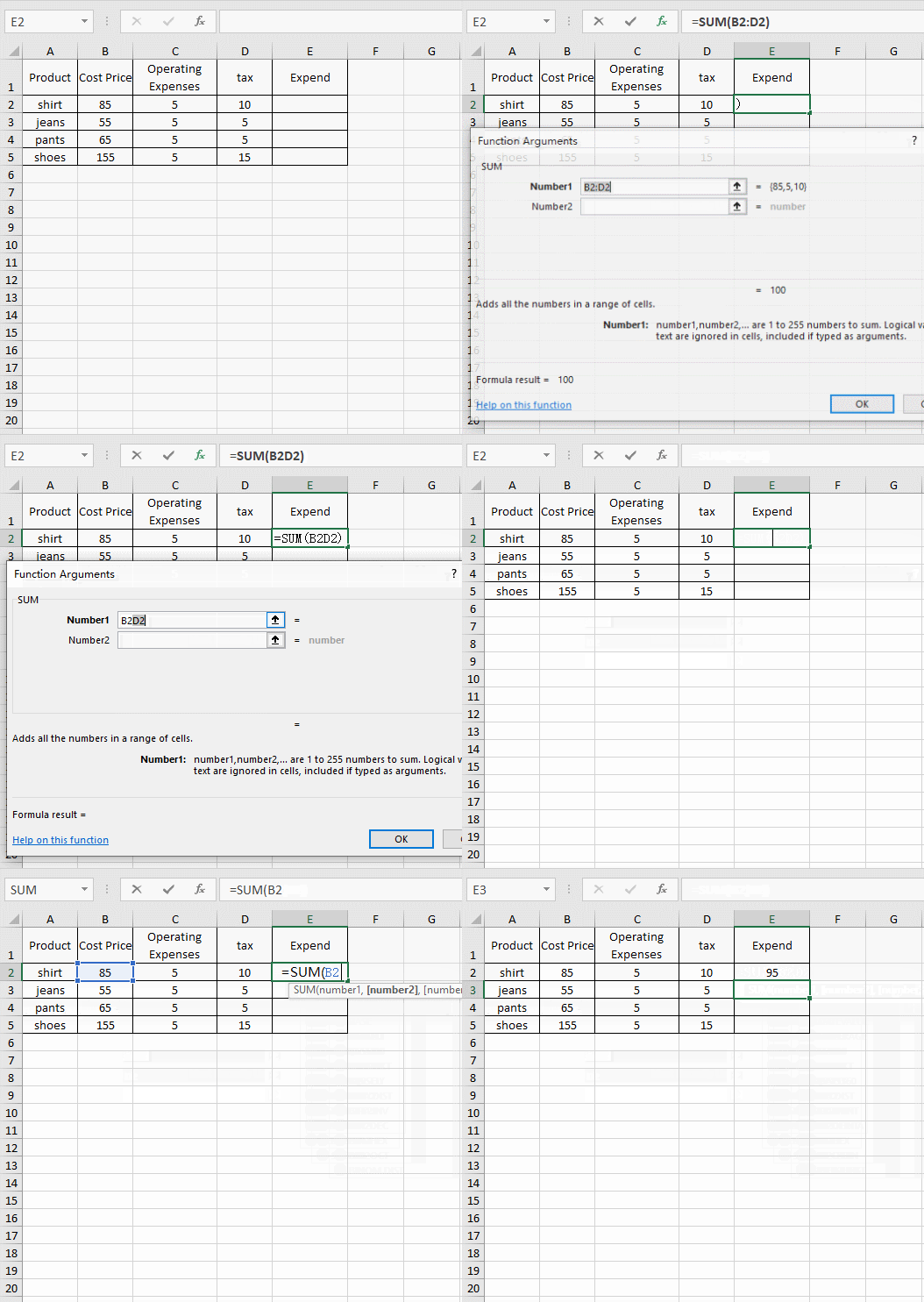
⑤ Hit OK, Excel will work the total amount out immediately.
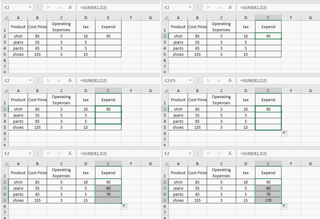
⑥ There’s one more small trick I want to share. If you want to apply the same formula in a range of cells, put your cursor at the right lower corner of the cell till it turns into a small black cross. Drag it to contain all the cells you want to apply the same formula.
2. Calculate Percentages
It’s frequent at work to make sheets involving percentages of different departments in a whole company. Calculating percentages with a calculator surely won’t take a lot of your time. But if there’re piles of data to deal with in a short time, Excel functions can definitely do a quicker job.
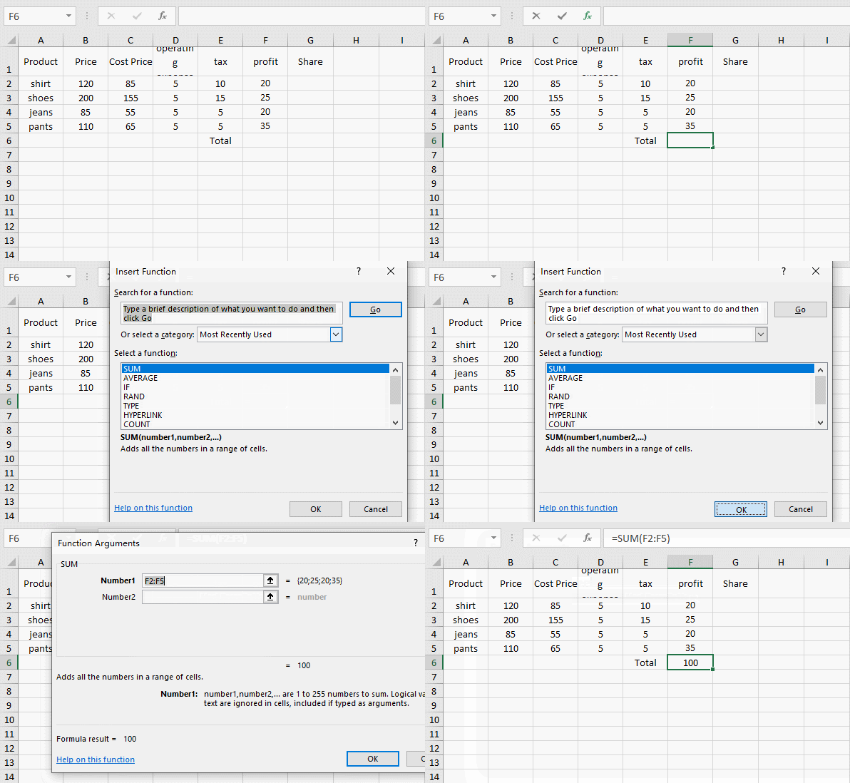
① To calculate the percentage, you must know the total amount in advance. Like the table below, the first thing I should do is to sum the profits from F2 to F5 with the method of using SUM function.
② Then click G2, and input the formula “=F2/$F$6“. F6 refers to the value in the B22, which is also the total amount of profits. And the symbol “$” makes it a fixed value. It won’t change even when we apply this formula to other cells.
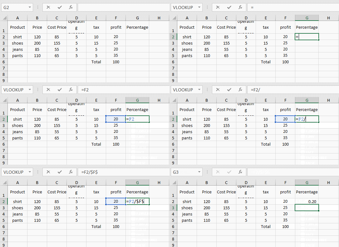
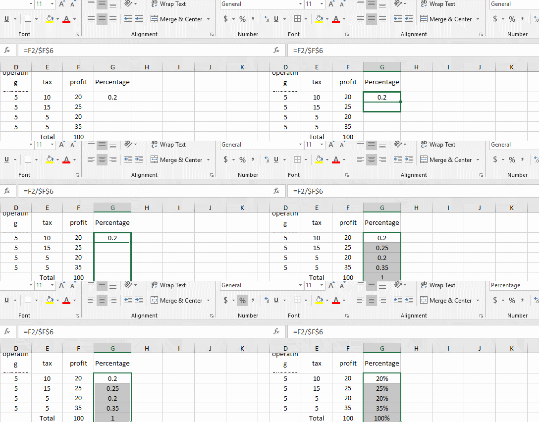
③ Press Enter key to work it out. Then with the trick I shared before, apply this formula to other cells in “Percentage” column.
④ If you want them to show as percentages instead of decimal fractions, just select all these cells and click the “%” icon in Home tab. The results will change into percentages immediately.
3. Evaluate the Average Value
Evaluating the average value is also a common need while doing calculations in Excel.
① Select a cell as the place to work the average value out, Click the icon of Insert Function – Averages, and then make your choice the poping out window of Function Arguments.
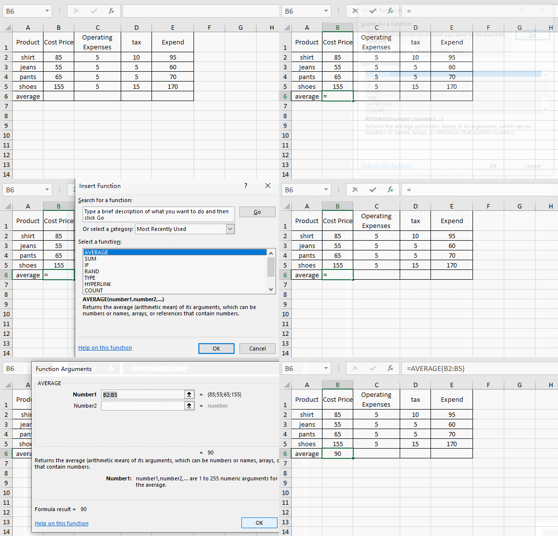
② Or you can input the formula “=AVERAGE(number1:number2)” directly. Here I want to evaluate the average value of the data from B2 to B5. So the complete formula is “=AVERAGE(B2:B5)”. Press Enter key and you can see the result.

4. Merge the Content in Different Cells
Sometimes you may need to merge the content from different cells in an existing table. If there’s a large amount of data for us to process in the table, Excel function can help you to save a lot of time and effort as well.
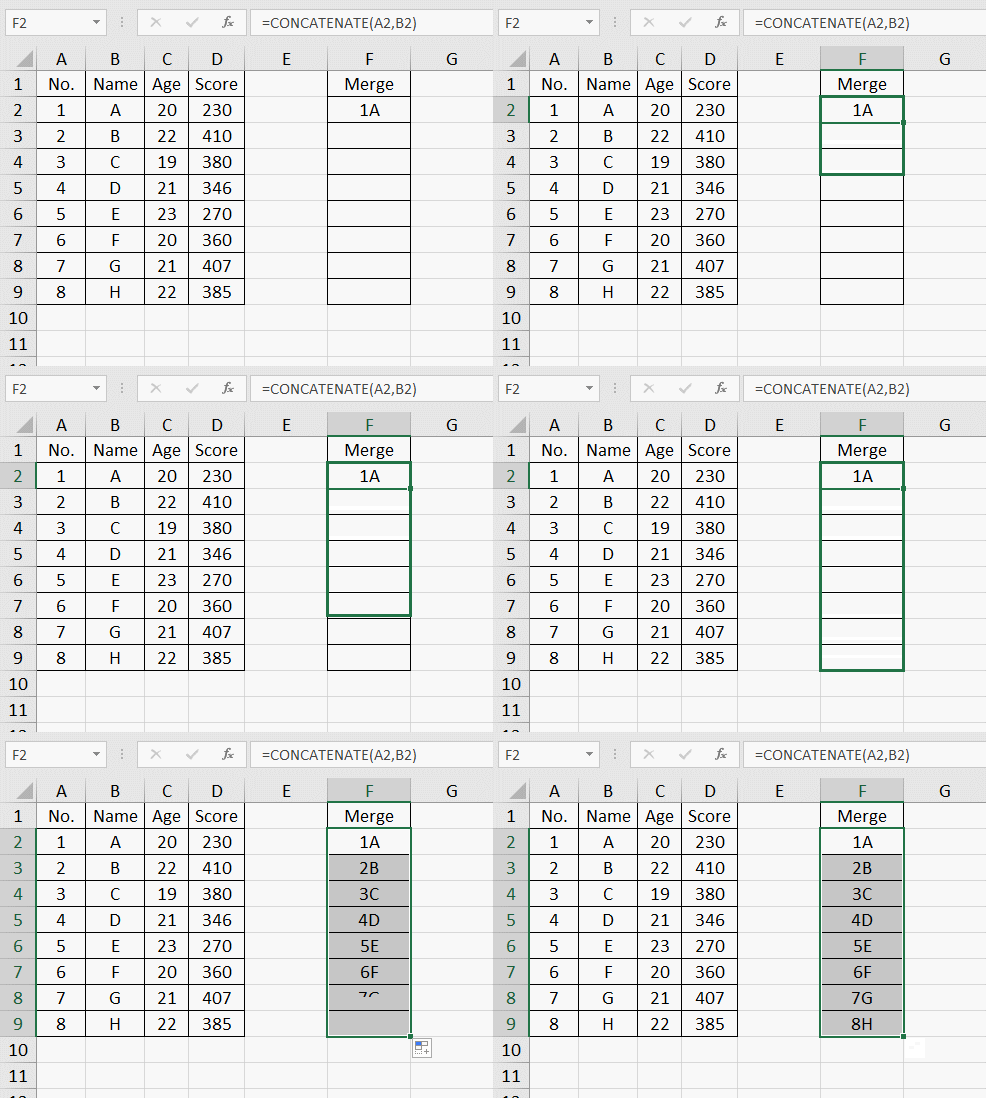
Like this table below, I’m required to merge the content of Column A and Column B in the new created “Merge” column.
① The first step is to merge the content of the first row in Column A and Column B. Input the formula “=CONCATENATE(A2,B2)” in F2 and then press Enter key. The text in A2 and B2 will be combined and filled in the F2 right away.
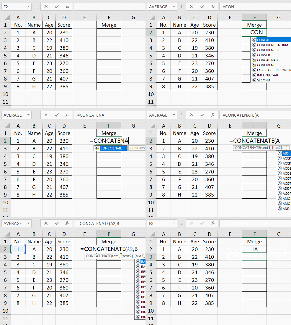
② Put the cursor at the lower-right corner of F2, it will turn to a small black cross. Then press and hold the left mouse, drag it to select all the cells in “Merge” column. Thus you can apply the same formula to a whole column, and the content from two columns will be merged successfully in a moment.
5. VLOOKUP Function
VLOOKUP can easily search through a column and find the corresponding data. For example, you can search for the score of a student in class quickly according to his or her name. It’s a very practical Excel function which can be massively used in work.
The basic formula for VLOOKUP is:
=VLOOKUP (lookup_value,table_array,col_index_num,range_lookup)
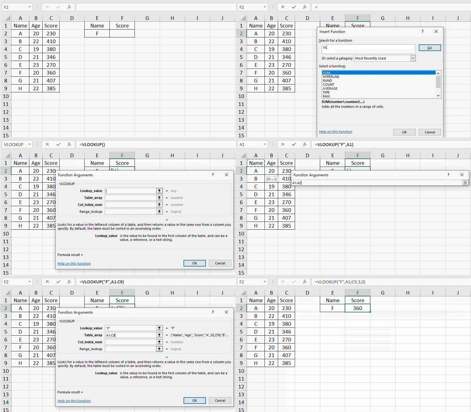
① Assuming there’s a long list of record in the table below. Now I want to find the score of someone, the first step should be inserting the formula correctly. So I click the cell I want to output the search result, which is F2 in my case, and hit the small icon of Insert Function.
② Type “VLOOKUP” in the textbox of Search for a function and hit Go. Click VLOOKUP in the section of Select a function and click OK to insert the formula (you can directly type it in the cell, of course).
③ Then you can input the value of each factor of the formula. For example, I want find the score of student F in the table, so the Lookup_value should be “F“. And the values of score are listed in the third column, so the Col_index_num should be “3“. Then set the Range_lookup as “0” for an accurate result.
④ As for the Table_array, a convenient way is clicking the small arrow on the right of the textbox, then hold and drag the left mouse to select all the cells in the table. The range of table will be inserted to the textbox accordingly.
⑤ Click that small arrow again to get back to Function Arguments window. Now all the textboxes have been filled up. Click OK to close the window. VLOOKUP function has already found the data I’m looking for in F2.
This is what I want to share for today, hope it can be a little inspiration to your work. In fact, except for the 5 useful Excel functions I mentioned above, there are many other practical functions and formulas can improve your efficiency of processing text and data. You can also give them a try in the future.
Left the repetitive tasks to machine, invest your energy in some more creative work!

Thanks a lot, it’s very helpful 🙂
Thank you, Amber.