After often using some products or shopping online, we will judge the products or the shopping service, usually apply the five-star rating. We can give the number of stars according to our experience! In fact, you can also make a five-star rating effect in Excel. Let’s get started.
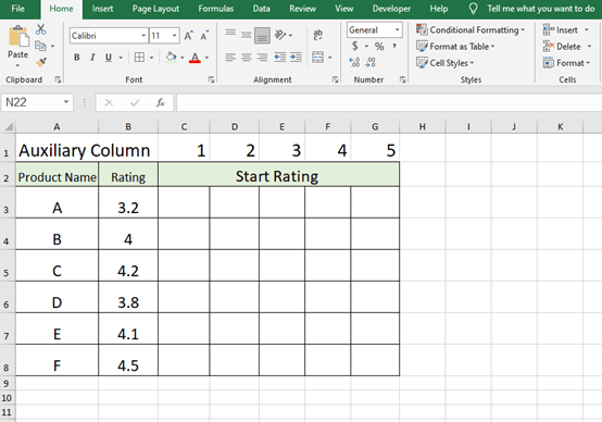
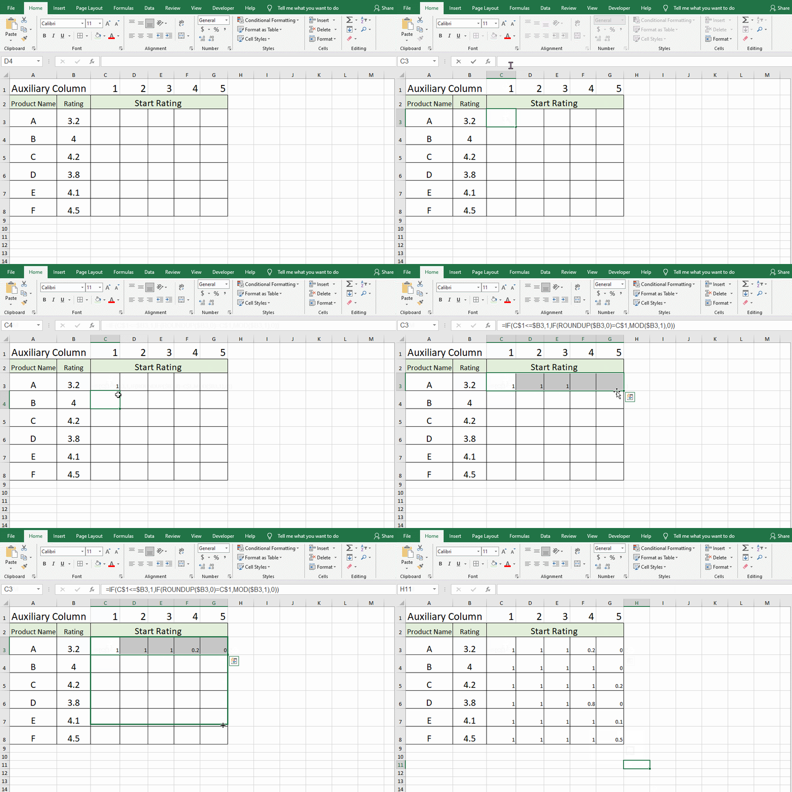
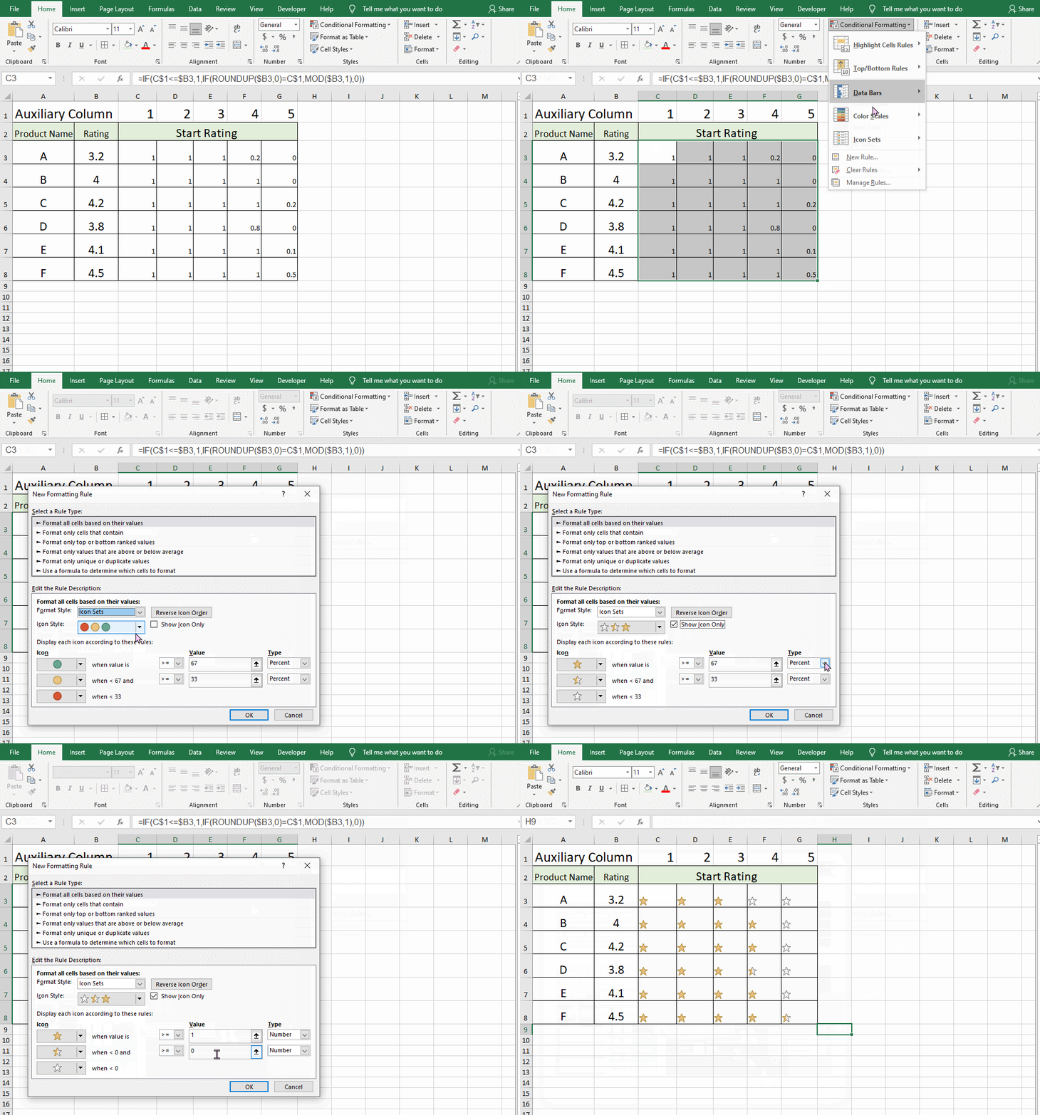
Step 1: Frist, we need to prepare a worksheet like below. Now we enter this formula in cell C2 and fill to other cells.
=IF(C$1<=$B3,1,IF(ROUNDUP($B3,0)=C$1,MOD($B3,1),0))
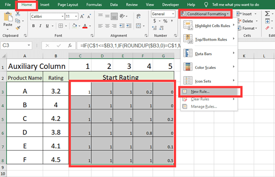
Step 2: Select the cells that need to be filled with star ratings first and click on Home in the toolbar and choose Conditional Formatting. Choose the New Formatting Rule to open the Window.
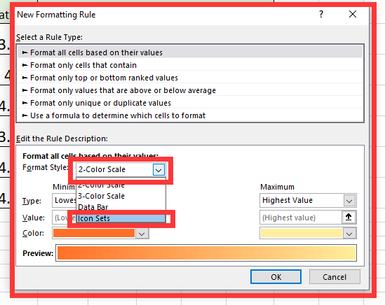
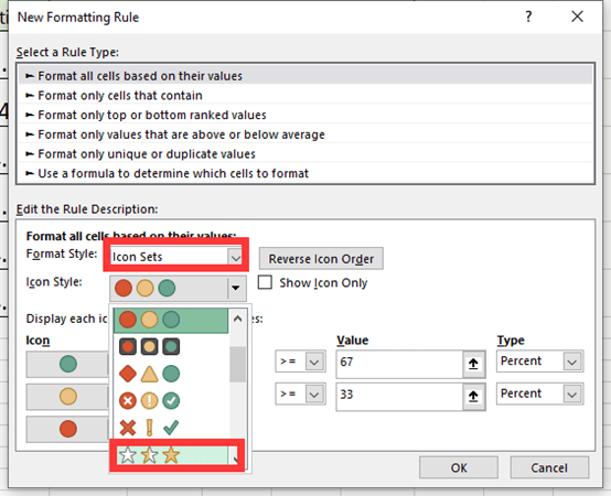
Apply Icon Sets to Format Style, and choose the last style: Three Stars.
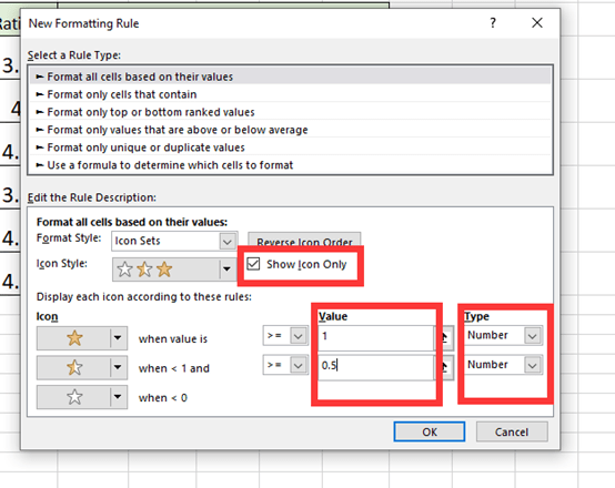
Check the box before Show Icon Only, and adjust the Value and Type like this picture below. Then click Ok.
Step 3:
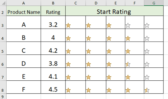
Hide the first Auxiliary row for better look. And adjust the table.
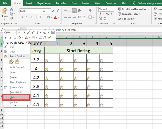
Now, you’ve got the perfect start rating effect!

Leave a Reply