There should be no one who doesn’t know how to use Excel’s filter function. But being able to use it does not mean “Efficient”. In many cases, because you don’t know the method, you will spend extra time on unnecessary steps. In today’s article, Sandra will introduce 7 tips of quickly selecting cell to everyone, so that you can spend 50% less time on Filter.
Tip 1: Ctrl+ Shift+ L
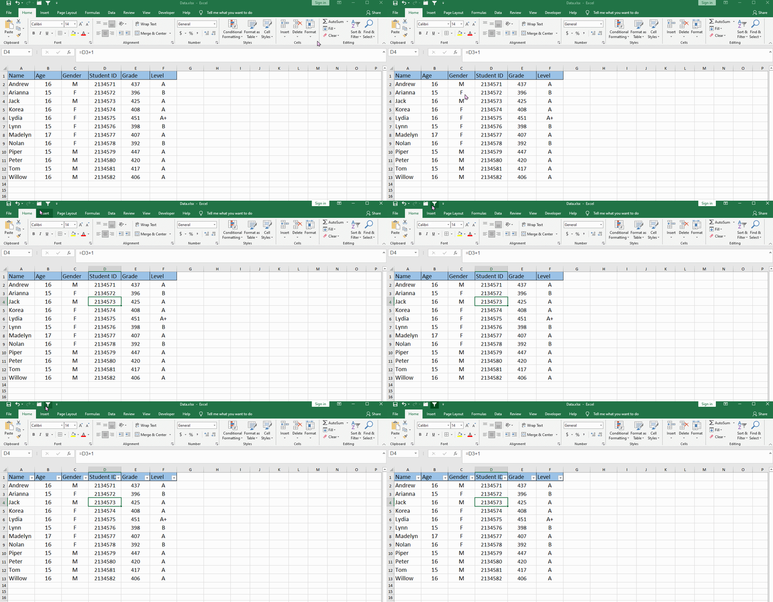
Click on any cell and use shortcut key Ctrl+ Shift +L.
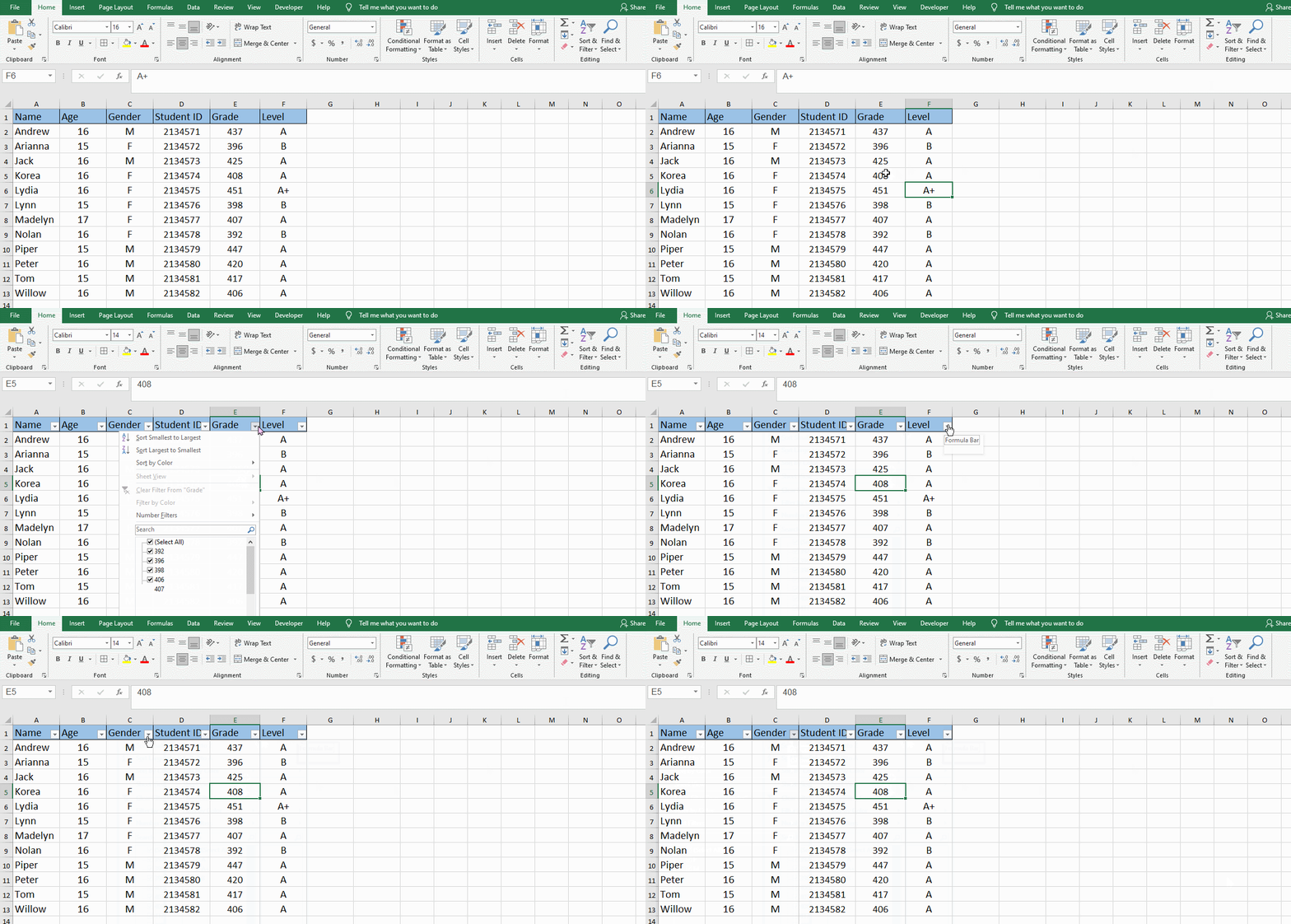
You can think of this shortcut as quickly opening the “Filter”.
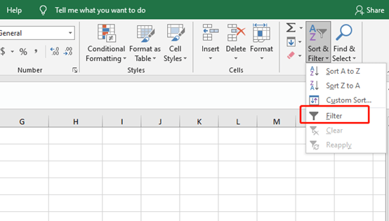
Tip 2: Add to Quick Access Toolbar
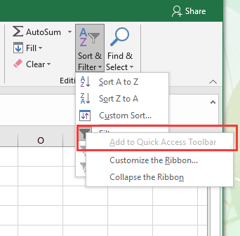
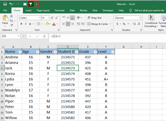
Right-click Filter and select Add to Quick Access Toolbar.
Tip 3:Right-Click to Filter Directly
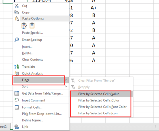
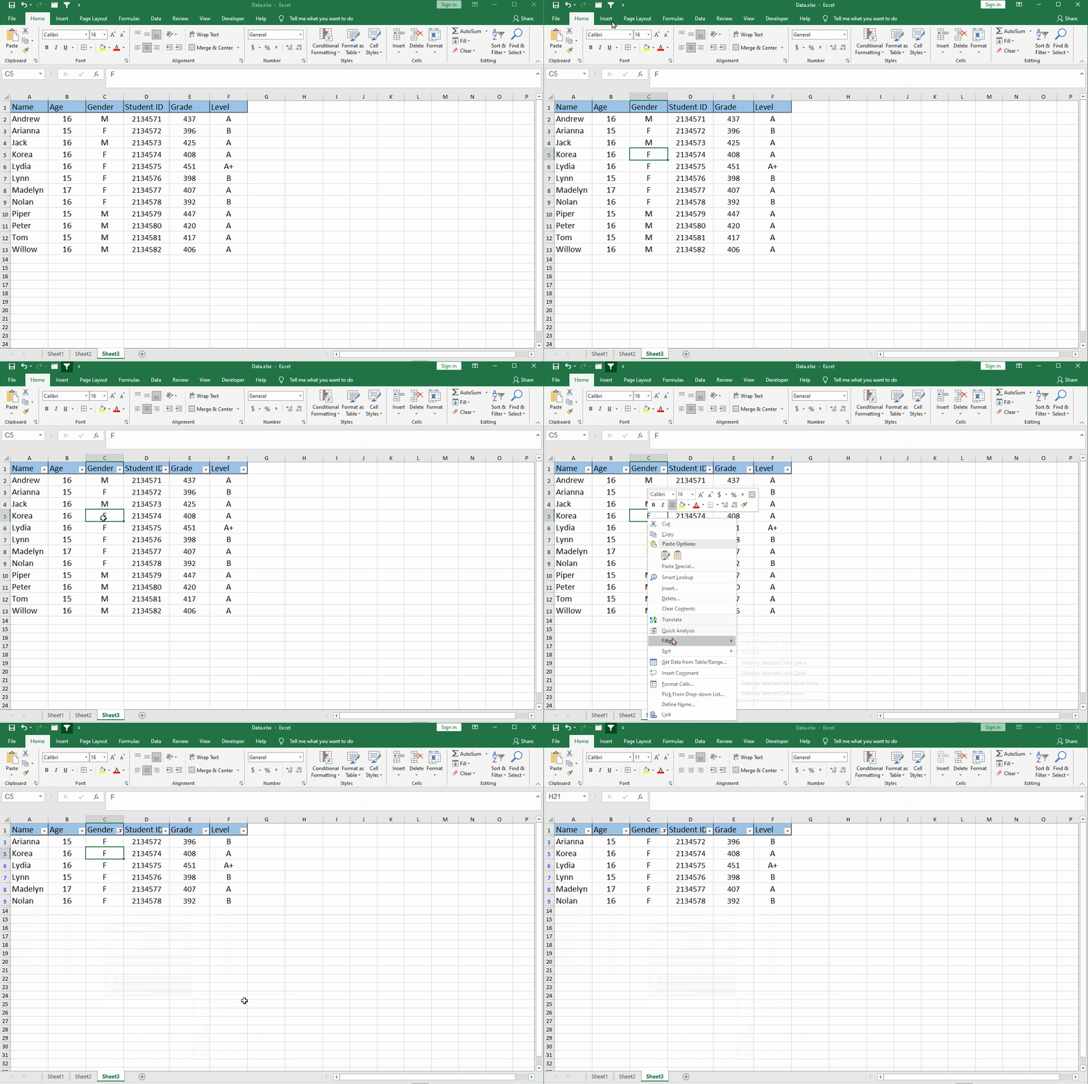
Select your aim value or color or Font color, and right-click to choose Filter by Selected Cell’s Value in the list. You can quickly get all the value you need in the range.
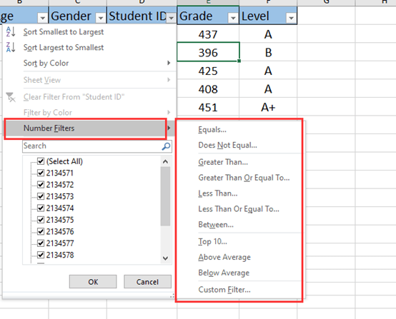
Tip 4: Detailed Filter
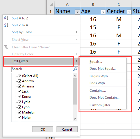
Microsoft Excel provides a variety of filter conditions for text, numbers and dates. You can use these conditions reasonably without requiring other complicated filter steps.
Tip 5: Search in the Filter
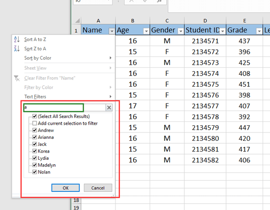
After the filter is enabled, click the filter arrow of the target column and enter the content you want to filter in the search box. Excel will filter the data that meets the conditions in real time according to the input content.
This trick is particularly suitable for situations where there is too much data in the sheet.
Tip 6: Use Wildcards
In Microsoft Excel, a wildcard is a special kind of character that can substitute any other character. So, when you do not know an exact character, you can use a wildcard in that place.
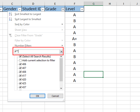
The asterisk (*) is the most general wildcard character that can represent any number of characters. For example:
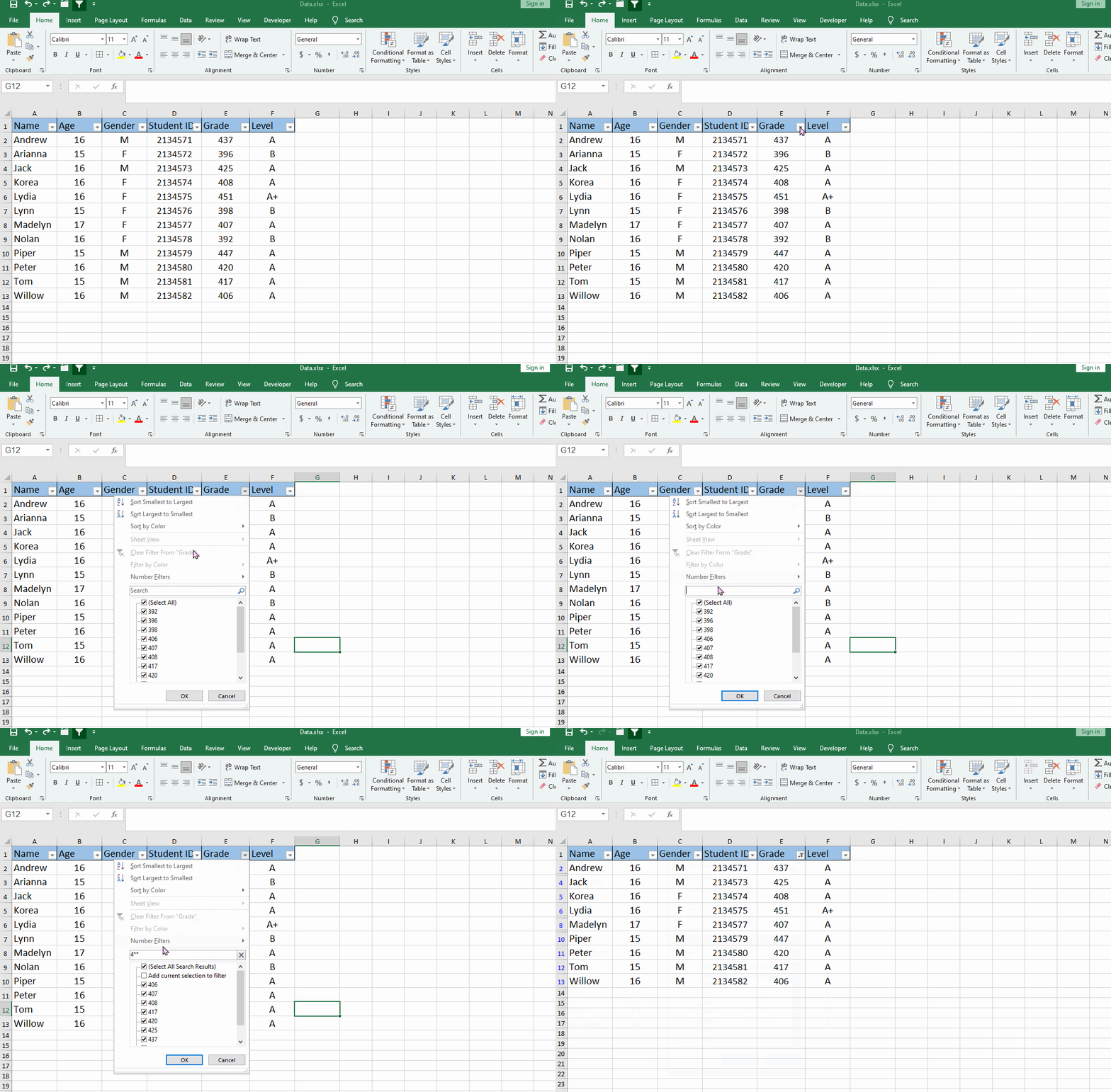
If you want to quickly get rows with a score of more than 400, you can enter “4**” in the search box.
The question mark (?) represents any single character. It can help you get more specific when searching for a partial match. For example:
If you want to know the grades of students whose names start with P and have eight letters. Then you can enter “P???????” in the search box.
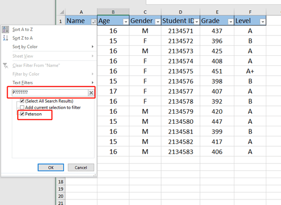
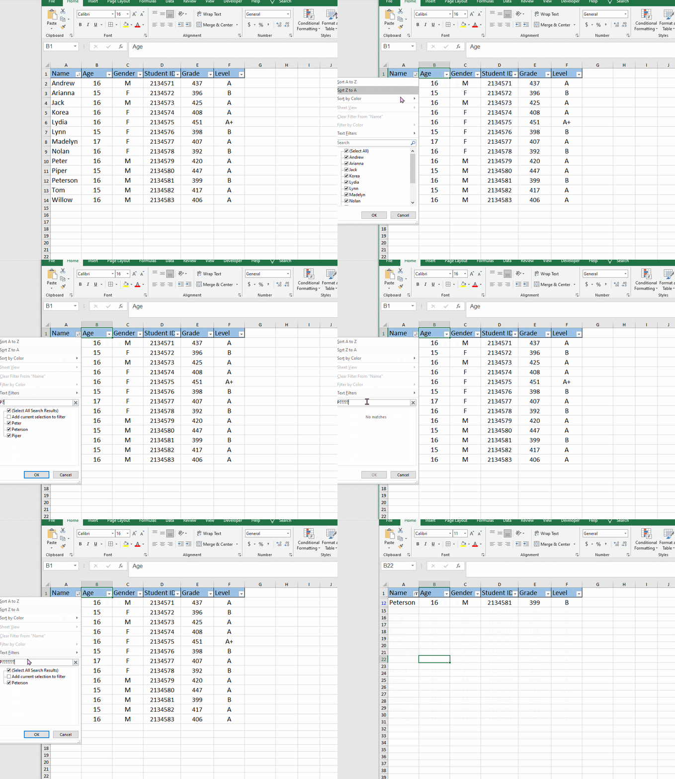
The tilde (~) placed before a wildcard character cancels the effect of a wildcard and turns it into a literal asterisk (~*), a literal question mark (~?), or a literal tilde (~~). For example:
Suppose you now need to search for cells that contain *.
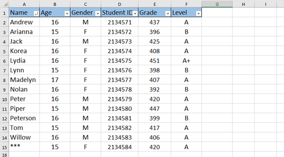
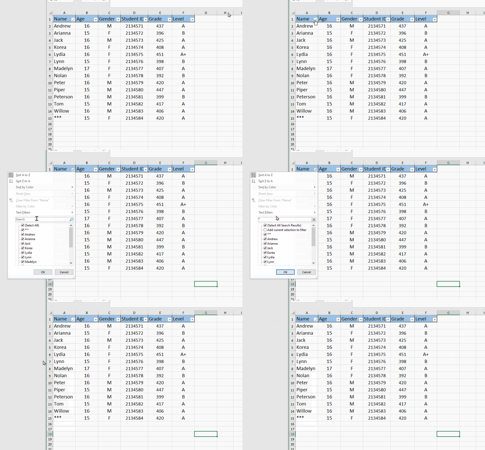
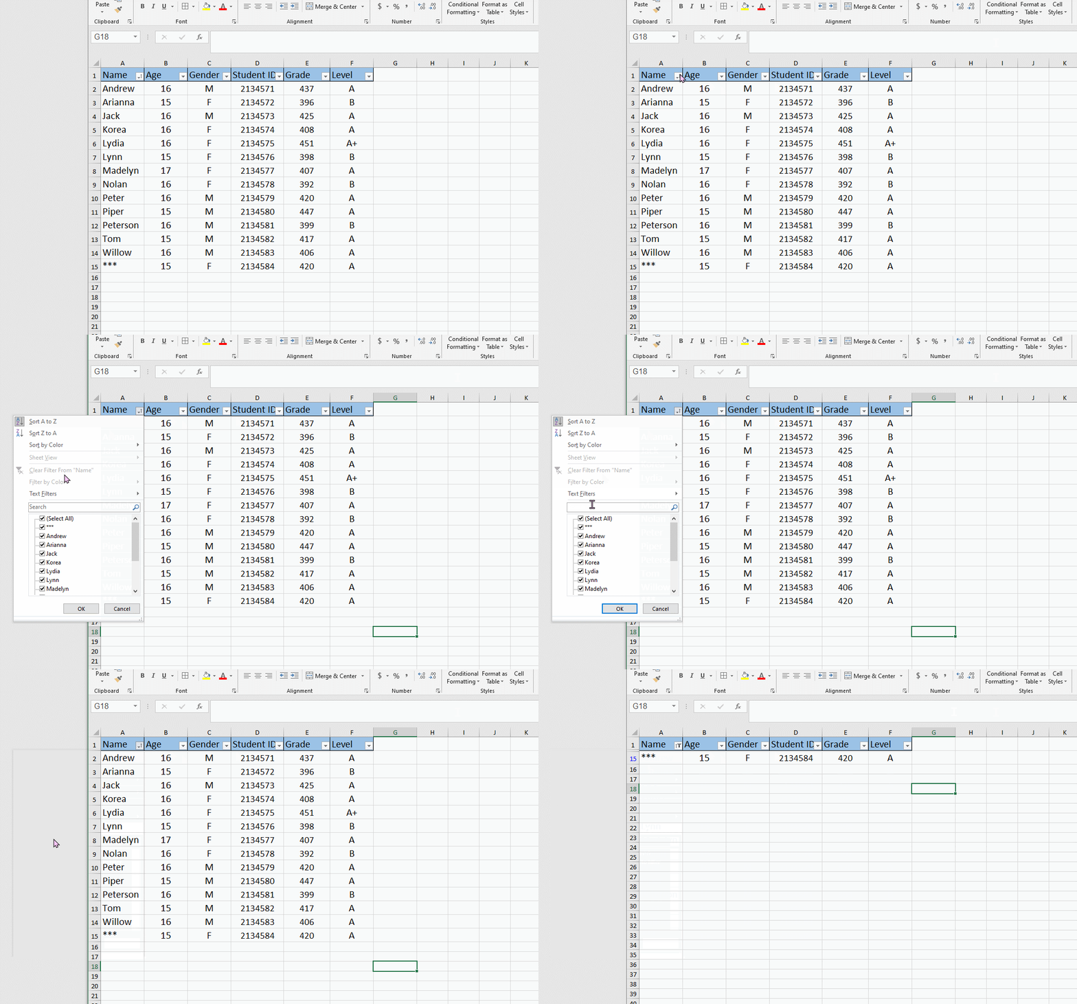
If you just search “***” or only “*” in the search box, you will find that nothing changed. But if you put a tilde before.
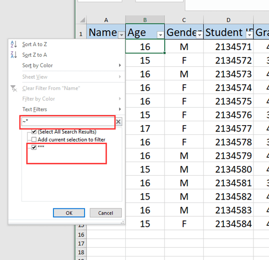
You can quickly get the value that contains” * “.
Tip 7: Slicer
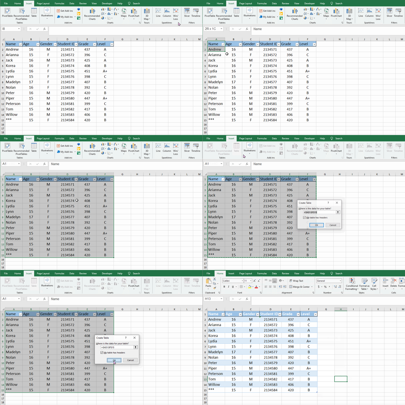
You need to change your date area into a table first, then you can use the slicer function.
Select the date range and go to insert tab, choose Table, or you can also use shortcut key Ctrl +T.
Now, you can go to insert tab and hit Slicer function.
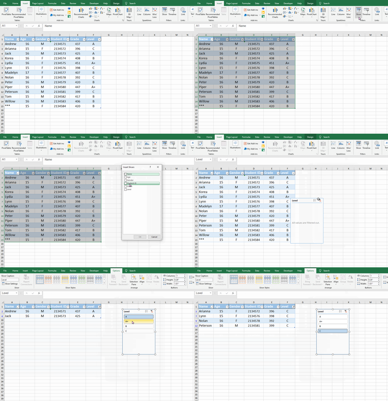
Using slicers can help us get the data we need more quickly, and we don’t need to click the mouse repeatedly.
As you can see, a simple data filter has so many tips to improve efficiency.
Okay, have you learned the above 7 skills? If you have other data filtering tricks, you can also leave a message below.

Leave a Reply