How to Add Borders in Excel Automatically in Two Conditions

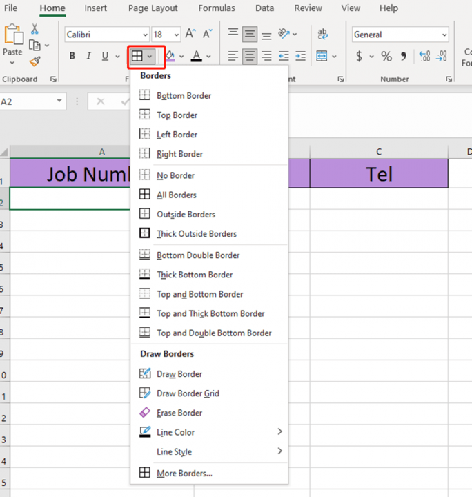
We usually select the cell(s) where we want to add the border firstly, then click the border list arrow from the Home tab to add borders. And click No Border to remove borders.

Today, we are going to learn a totally different and useful way to add or remove borders automatically.

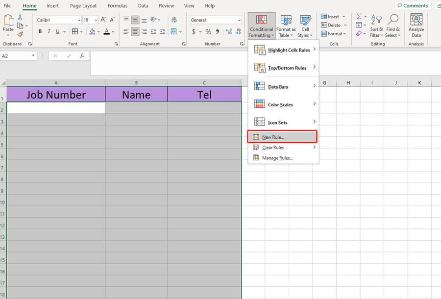
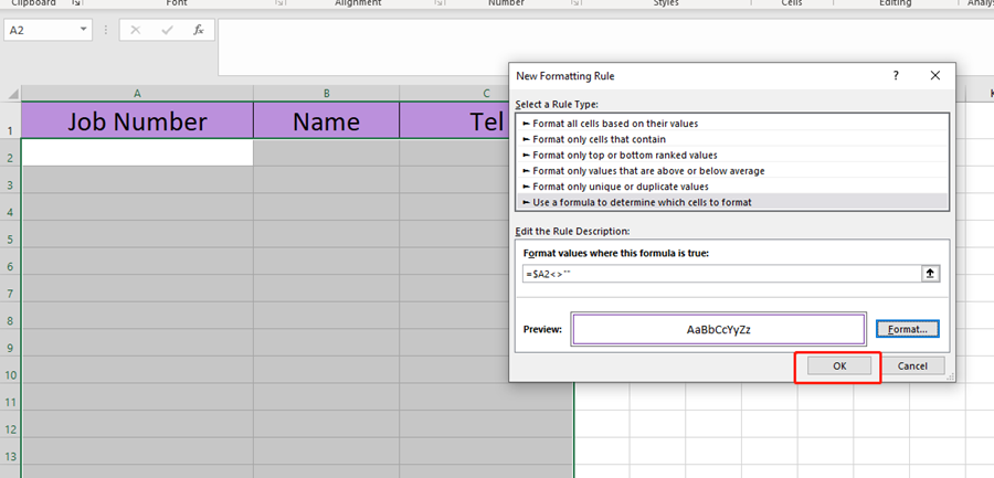
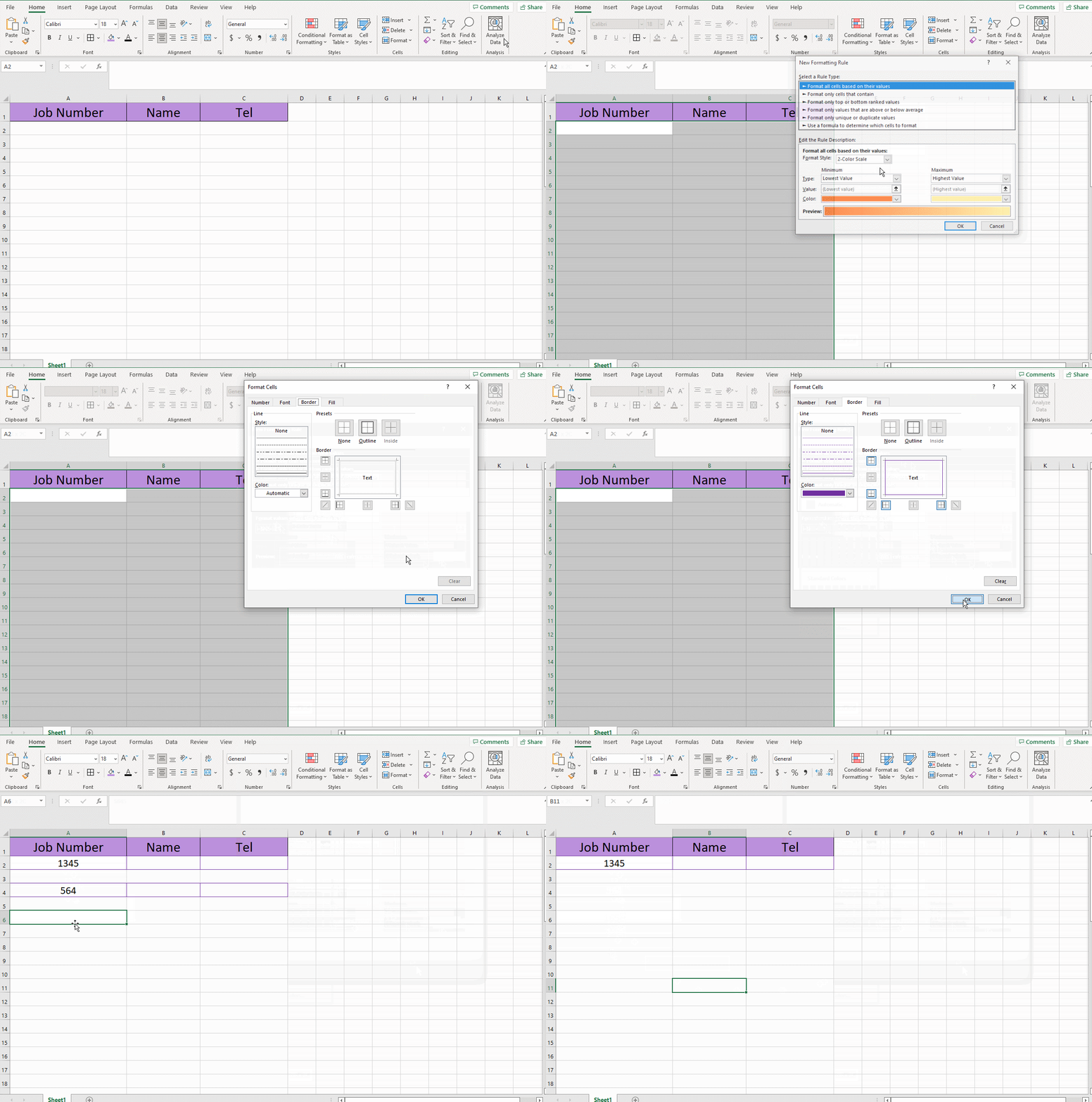
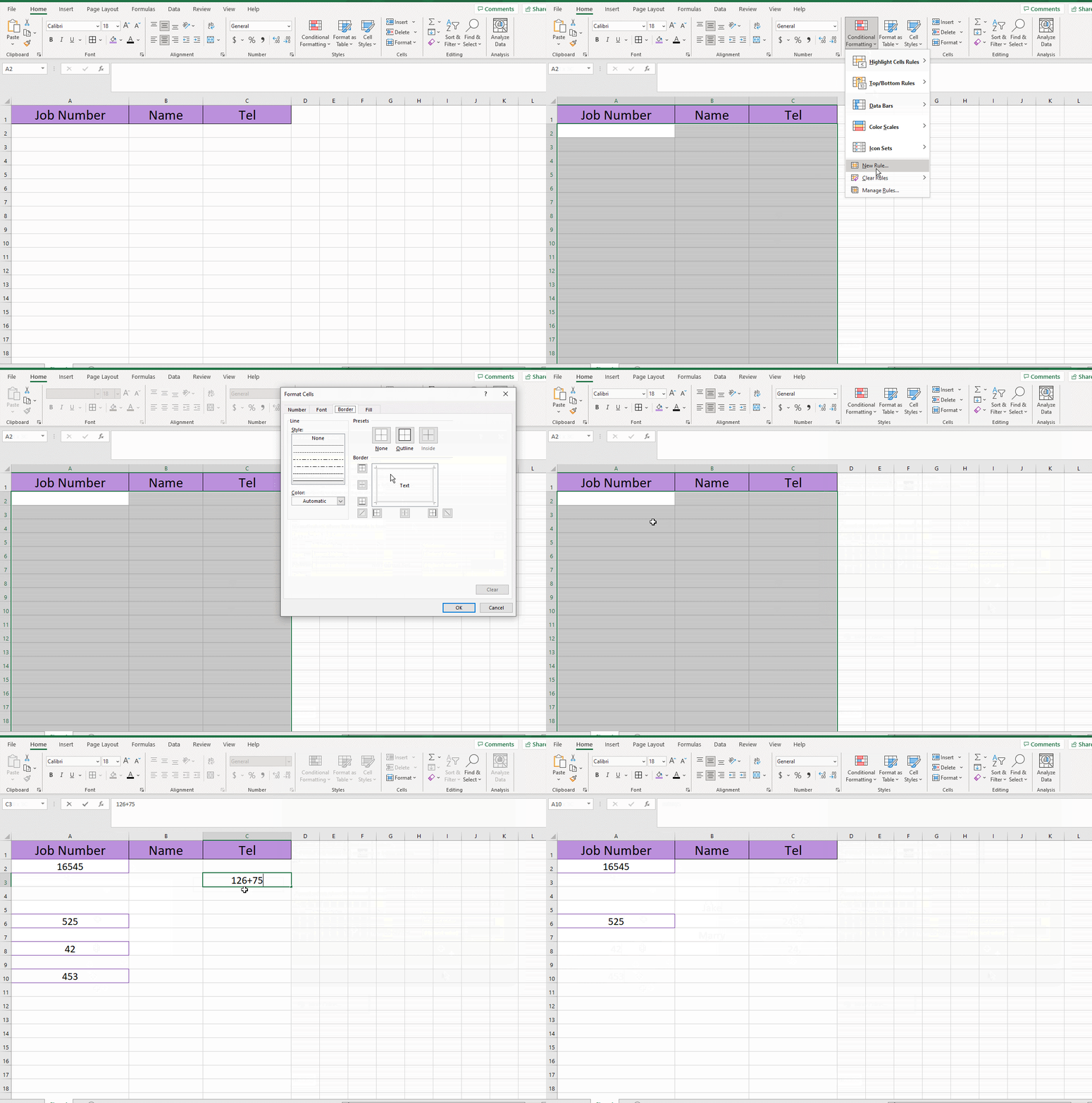
We first select the area from A2 to C20, then click the arrow of Conditional Formatting, and choose New Rule.

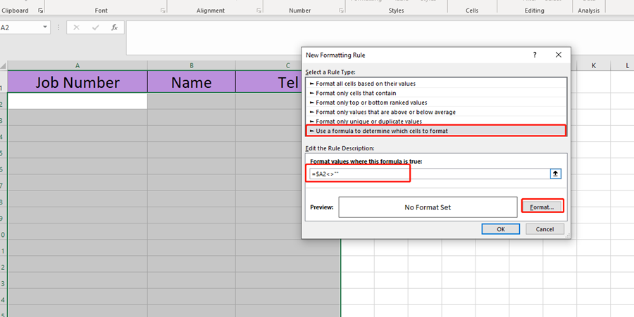
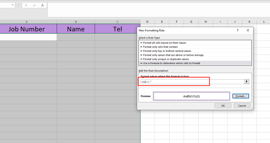
Select the last choice, Use a formula to determine which cells to format.

Edit[ =$A2<>” “] in the box and click on Format button.

<>: it means not equal to.

” “: it represents a null value.

We set the outline border and color.

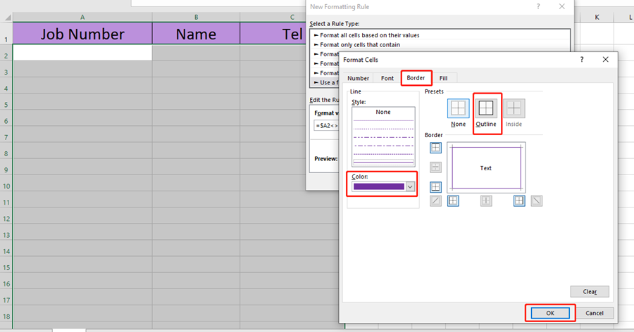
Hit Ok.

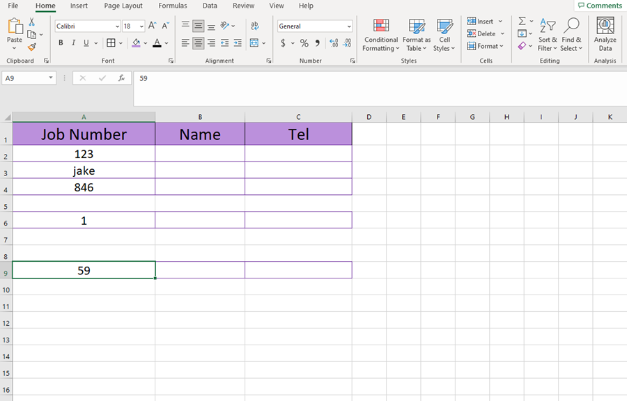
Now, when you enter any data or content in column A, there would show borders from row A to C. If you delete the content, the border would be removed automatically.

If you only want to add borders to the cell which has content.  You can just change the [=$A2<>””] into [=A2<>””]

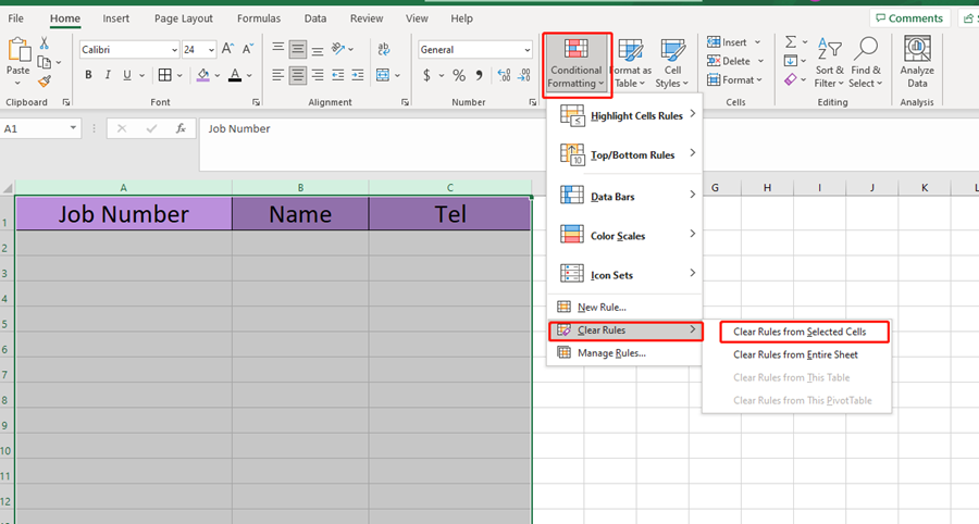
That’s more useful and effective than adding borders from the Home tab.