Calculating the average value is a very common way to analyze data in Excel. To do the computations accurately and also rapidly, you can use Excel function to calculate mulitple, or even an entire column of data. Here’s the basic approach to use AVERAGE functin.
1. Select the E2 cell, Click Formulas – AutoSum – Averages (or you can input “=AVERAGE(B2:D2)” directly).
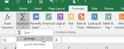
In this formula, B2:D2 refers to B2 to D2 (including C2), the range of cells you want to evaluate.
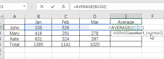
2. Press [Enter] key and you can see the result.
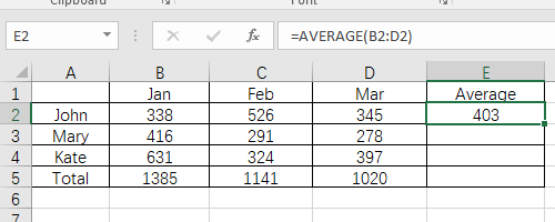
3. If you want to evaluate the average value in E3, E4 and E5 as well. Don’t bother to input the formula in each cell. Just click the lower right corner of E2 till the cursor become a black cross, drag it to contain all these cells. The average formula will run in each of them automatically.
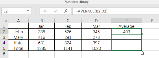
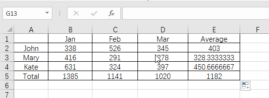
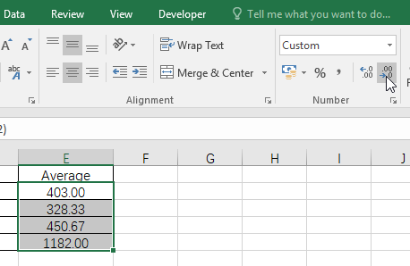
4. If you think there’re too many decimal digits, choose the cells and find Increase Decimal and Decrease Decimal in Home tab.
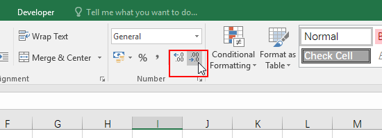
Use these two button to customize the decimal digits in the sheet as you like.

Your style is so unique compared to many other people. Thank you for publishing when you have the opportunity,Guess I will just make this bookmarked.2