How To Check The Checkbox To Change The Cell Color

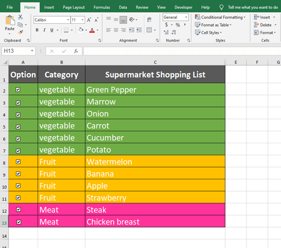
This is a very cool effect in Excel. When you checked each checkbox, the color of the related row would be changed at the same time.

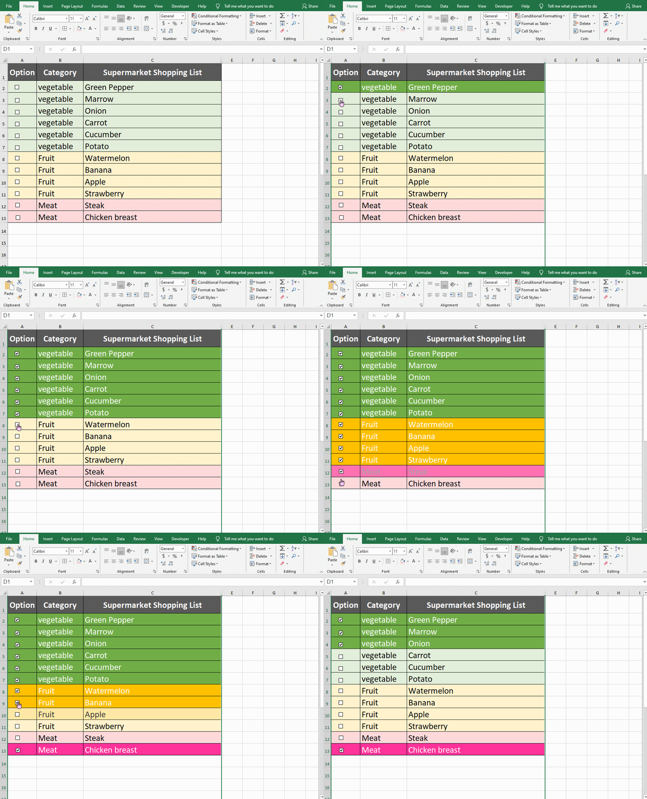
Ok, let’s get started. The content of this tutorial may be a lot, but it is not complicated. The author suggests you open an Excel sheet to have a try.

Step 1: Create the Basic Part of Table

Prepare the basic part of the “Supermarket Shopping List”. Of course, you can create others. This step would be easy if you always use Excel in your daily work. You can choose the colors you like as Fill color, but light colors would be better.

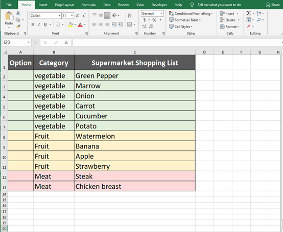
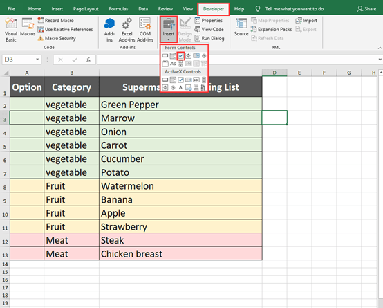
Step 2: Insert Controls

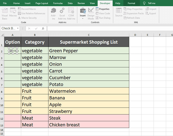
Go to Developer and click on Insert. Choose check boxes in the list.

You can delete the “Check Box 1” text to looks more beautiful.

We consider column D as an auxiliary column, and enter TRUE in this column except title row.

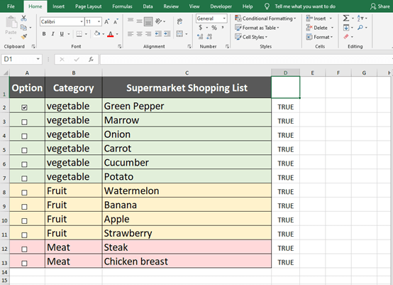
Step 4:  Create Cell Link

Check the first checkbox and right-click on the checkbox, choose Format Control.

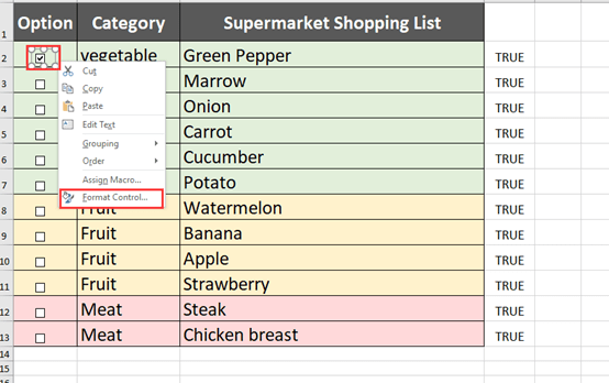
Make this checkbox in A2 link cell D2. Repeat this step for every checkboxes.( Checkbox in A3 cell link D3……)

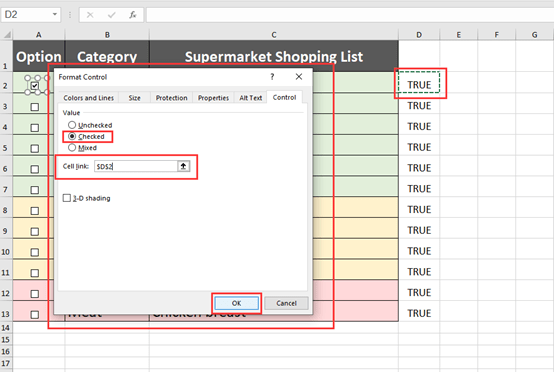
After this step, you will find that when the checkbox is checked, the related D value will display TRUE, If it is not checked, the value FALSE will be displayed.

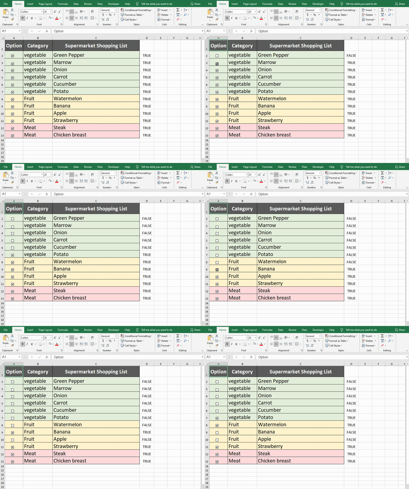
Step 5: Create New Formatting Rule

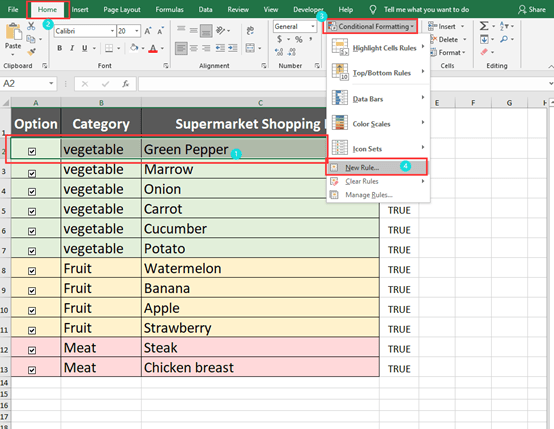
Highlight A2 to C2 first and go to Home and click on Conditional Formatting in the toolbar, choose New Formatting Rule in the list. And then Choose the last option “Use a Formula to determine which cells to format” in the New Formatting Rule window.

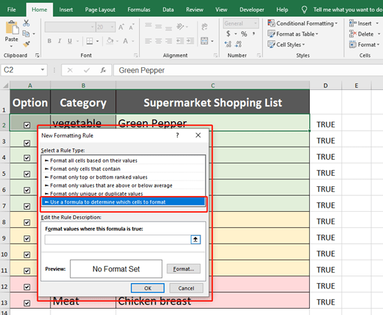
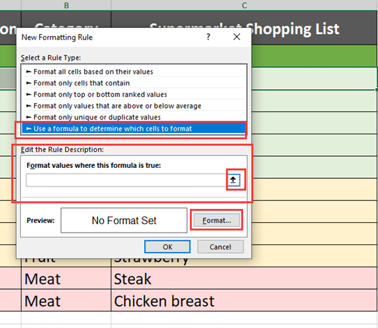
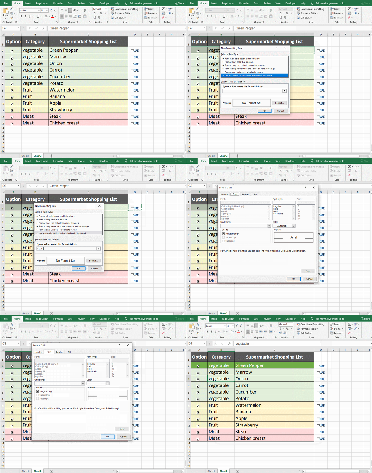
Now, you need to edit the rule description like the GIF below. Do these settings for each row.

Step 6: Hide the Auxiliary Column

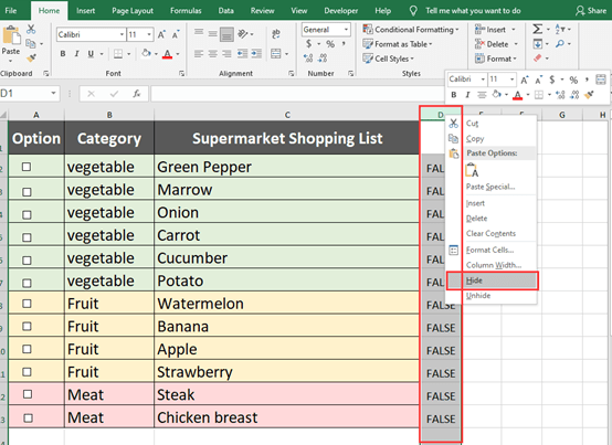
Select the column D and right-click it, choose Hide in the list. It’s just for a better look.

Now, you have finished all the steps. That’s really cool.