A large table with tons of data usually can’t be fully displayed in a single page. You must scroll down or scroll to the right for a more complete viewing. In order to correspond these data with the title or other key content intuitively, you can freeze some specified cells in the table. In this way, even when you scroll down the page, the selected content will always show at the top of the page.
How to Freeze Top Row and First Column in Excel
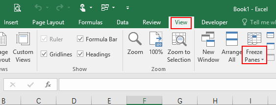
1. Switch to View tab in Excel, find the feature called Freeze Panes in the Window section.
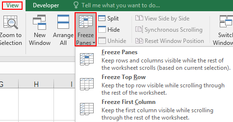
2. Click it, there are two common used options: Freeze Top Row and Freeze First Column. As their name suggest, you can simply freeze the first row or the first column in the table by selecting them.
How to Freeze Specified Cells in Excel
If you want to freeze a specified area of cells, you’d better make use of the feature Freeze Panes.
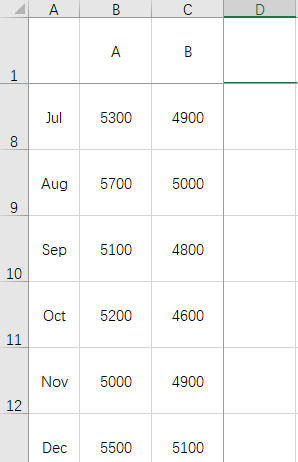
Freeze Panes allows you to freeze a specified range of cells, but not in a direct way. When you click a cell, the intersection of cells above it and cells on the left of it will be specified as the panes to freeze. For example, when I click D2 in the table and select Freeze Panes, the cells from A1 to C1 will be frozen. You can see the black borders around them which delimits the scope of cells to be frozen.

Now when I scroll down the page, the cells above the horizontal border line will always stay at the top of the sheet; When I scroll to the right, the cells on the left of the vertical border line will always stay at the leftmost of the sheet. And no matter I scroll down or scroll to the right of the page, cell A1, B1 and C1 will always stay at the same place.
How to Unfreeze Panes in Excel
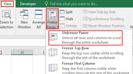
If you don’t want to freeze these cells anymore, just click Freeze Panes again and choose Unfreeze Panes in the drop-down list.

Leave a Reply