If you entered a series of dates into Excel spreadsheet, and want to highlight all the nonworking days. Do you have to pick out the weekends manually?
In my previous post, I’ve introduced some uses of the powerful Conditional Formatting. It enables you to apply a format to multiple cells that meet the specific criteria. In this case, it can also help you to highlight all the nonworking days in a spreadsheet automatically.
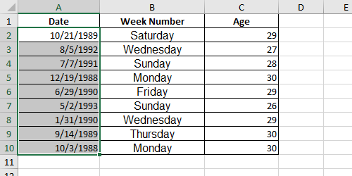
1. Select all the cells with dates.
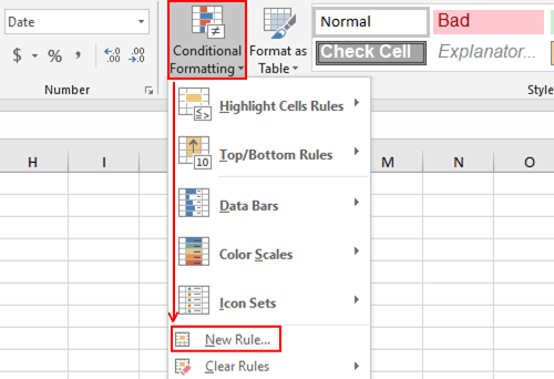
2. Click Conditional Formatting in Home tab and choose New Rule… in the drop-down list.
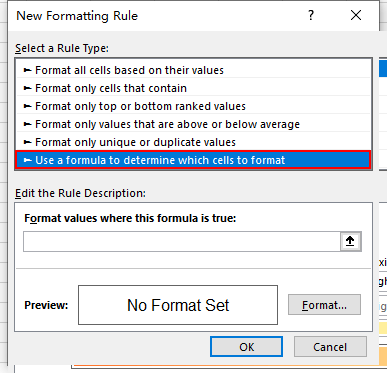
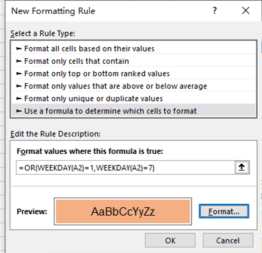
3. Switch to Use a formula to determine which cells to format in Select a Rule Type.
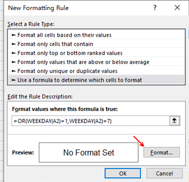
4. Enter this formula in the textbox under Format values where this formula is true: =OR(WEEKDAY(A2)=1,WEEKDAY(A2)=7)
Then hit Format… button at the lower right corner.
Please note: in this formula, A2 refers to the first cell of the selected range, you can change it according to your actual situation.
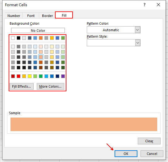
5. In the Format Cells window, switch to Fill tab and choose a color you like. Click OK to confirm the choice.
6. Hit OK again in New Formatting Rule.
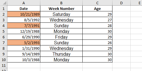
7. Now all the nonworking days in this table have been highlighted with the color you chose.
Alternately, you can use Filter to achieve the same goal without Conditional Formatting.
1. Use the formula: =TEXT(A2,”AAAA”) to calculate the week number in a new column at first.
You can check the detailed steps in the post about Excel tips for beginners (the 23th point).

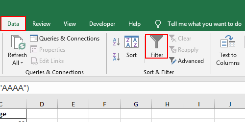
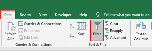
2. Select the entire column of Week Number (including the header) and Go to Data tab, choose Filter.
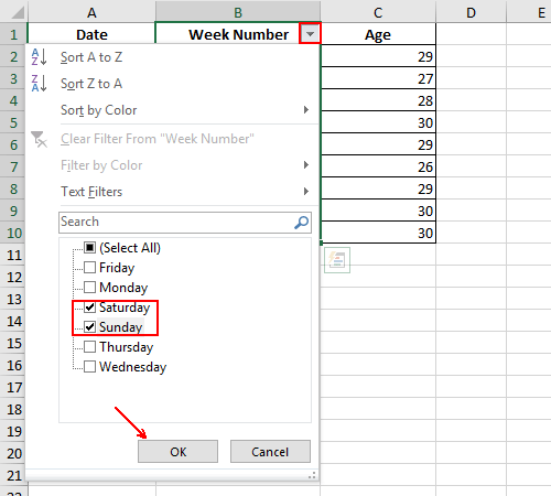
3. You will find a small triangle beside the first cell in the selected range. Click it, check only Saturday and Sunday. Then hit OK to confirm it.
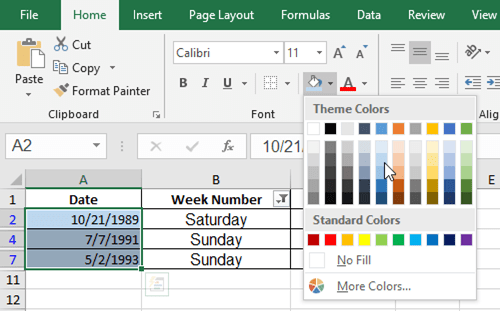
4. Then you can select all the cells left in the Date column and highlight them with the color you like.
5. Then click Filter in Data tab again.
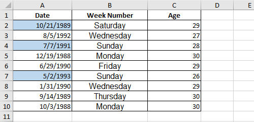
6. Now all the dates of nonworking days have been highlighted.

Leave a Reply