How to Insert Sparklines (mini charts) in Microsoft Excel

Sparklines are the mini charts in Excel cells that using simple and small graphs to present the status of data intuitively. Let’s see how to create and insert a sparkline inside a specific cell.

The sheet below shows the incomes of A and B from January to December. Now I want a more intuitive view of the variations. So I choose the cell N2 as the location to output the mini chart for A, and N3 for B.

1. Select the cell N2. Switch to Insert tab and find Sparklines section.

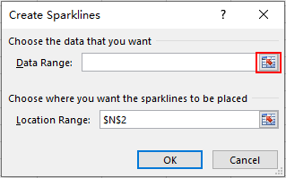
2. Choose a type suits your situation. In my case I chose Line, and click the small icon besides the textbox of Data Range in Create Sparklines window.

3. You can then drag the mouse to select the range of data you want the chart to contain.

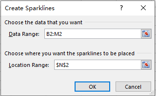
4. Click the icon beside the textbox again. You’ll be back to the Create Sparklines window and the textbox of Data Range is already filled.

Hit OK to apply the settings to your sheet.

5. Then the mini chart will be created in the selected cell N2 immediately.

6. You can still edit it in Design tab like adjusting the data range, chart type or style.

7. If you think the small chart is not intuitive enough and want to make the focal points stand out, try checking different points in Show section.

For me, I choose to emphasize the High Point and Low point. You can also check Markers to add point to the data of each month.

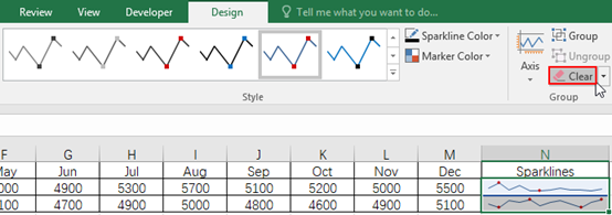
8. Please note the Sparklines added in this way can’t be deleted directly. But you can select them and simply click Clear in the Design tab. Thus they will be removed right away.