Usually we insert different kinds of data (like number and text) into different Excel columns for better recording the information and doing calculations. But sometimes we may also need to merge the content from different cells in an existing table. If there isn’t a large amount of data for us to process in the table, well, we can cut the content of a cell and paste it to another one by one. Otherwise it can be a tough task consuming a lot of time.
In this case, Excel function can help us to save time and energy as usual. A simple formula can do better and quicker than manual work.
Like this table below, I’m required to merge the content of Column A and Column B. So I create a new column called “Merge” in column F.

1. The first step is to merge the content of A2 and B2. Input the formula “=CONCATENATE(A2,B2)” in F2 and then press Enter key.
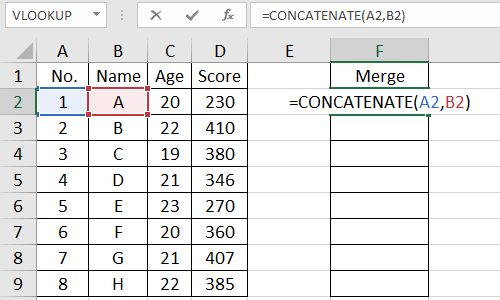
2. The text in A2 and B2 will be combined and filled in the cell F2 immediately.

3. Put the cursor at the lower-right corner of F2, it will turn to a small black cross. Then press and hold the left mouse, drag it to select all the cells in F column (which you want to output the result of merging) .

4. Release the mouse, now the formula is applied to all the cells you selected. In this way you can simply merge the content from two columns no matter how long the table is and how many data it contains.

5. This formula is not limited to merge the content in the same row. For example, if you want to combine the text of column A and the text in the next row of column B, you can complete the formula as “=CONCATENATE(A2,B3)” and input it in F2.
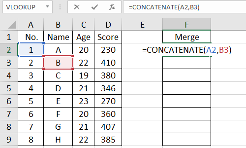
6. Press Enter to get the result.

7. With the method I shared before, apply this formula to all the cells in column F. It still works well.

8. Next time you want merge the content in different columns, try this function. It will doubtlessly save a lot of your time and effort.


Leave a Reply