When editing data in Excel spreadsheet, there may be some less important content you can’t delete but also don’t need to keep an eye on all the time. Hiding these rows or columns could make the table looks more compact without substantial impact for the data, and that’s exactly what I want to share in this post.
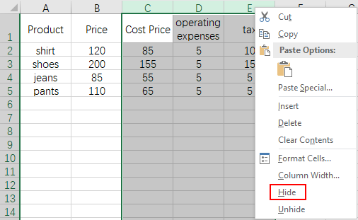
Take this table as an example. If I only want to compare the price and profit of each product, I can hide column C, column D and column E.

1. Select these columns by dragging the cursor from C to E in the area of column header, or you can hold down Ctrl key and click C, D and E on the column header separately.

2. Right-click selected area and choose Hide in the menu.

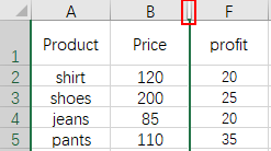
3. Then these 3 columns will be hidden while a mark with double vertical lines appears.

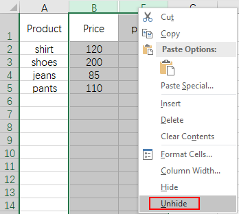
4. To view these columns again, just select the columns on both sides of the mark (In my case they are column B and column F). Right click your mouse and choose Unhide.

5. Then these previously hidden columns will show again.

You can also hide/unhide specific rows in the similar way.

Leave a Reply