Sometimes we highlight value or important data in different colors for different purposes. If we need to use color ranking or sort by color in Excel. What should we do?
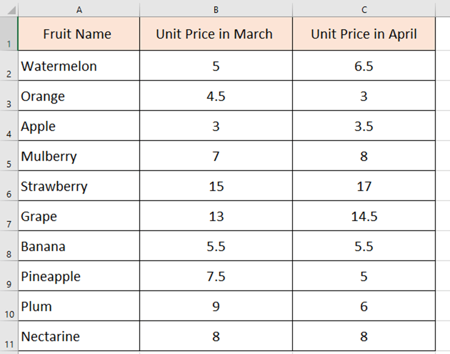
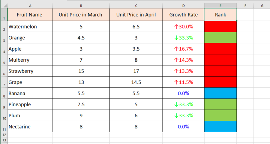
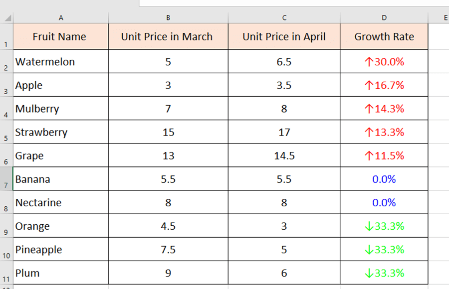
There is a price table for fruits. We can see that the prices in March and April are different. So, we can get the growth rates.
Do you still remember how to calculate the growth rate? We’ve talked about this in one of our previous tutorials. (How to Highlight the Growth Rates in Excel?)
Growth rate =Starting value– End value/starting value.
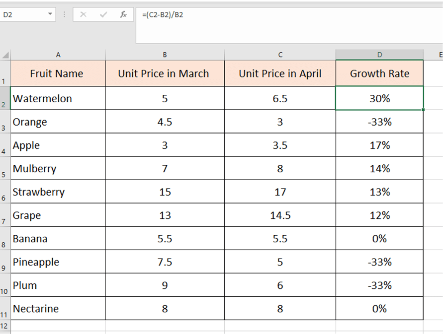
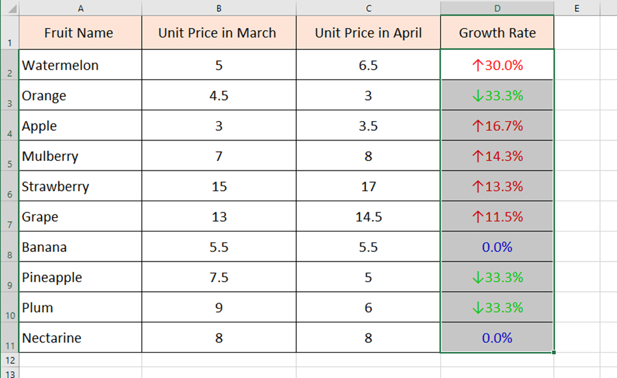
Then we highlight these growth rates in three colors. Red for growth rates; green for negative growth rate and blue for zero growth.
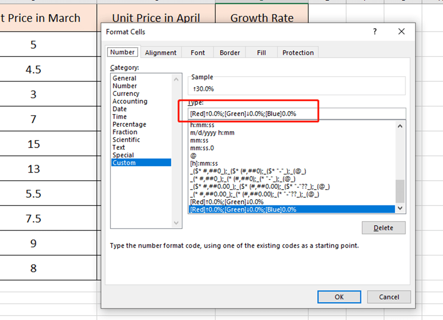
Select the area of the growth rates and go to the Alignment settings.
Choose the Custom behind Number and type [Red]↑0.0%;[Green]↓0.0%;[Blue]0.0% in the box. Then hit Ok.
The part before is just a review. Let’s move to the next part. How to rank by selected color?
We first made a helper column like the below.
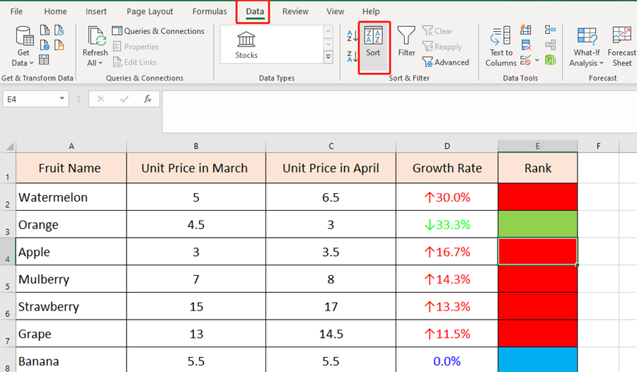
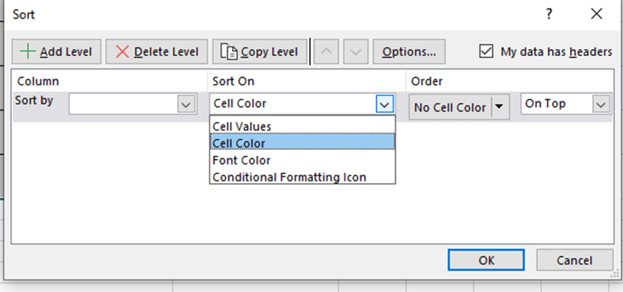
Then click any single cell of the Rank list to choose Sort.
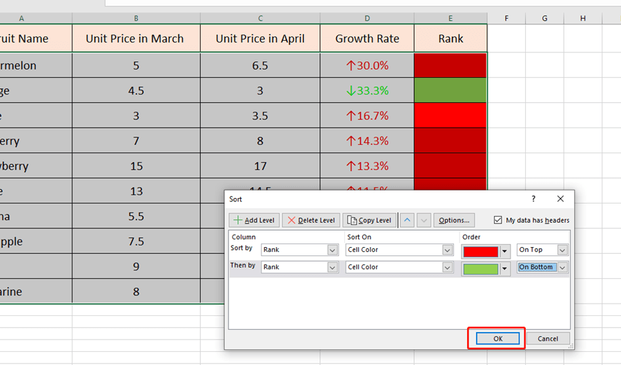
You can choose the color order as you like.
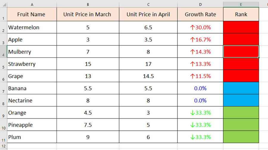
Delete the Rank list at last. You can also use this way to sort by color of the font.

See you guys next time~

Leave a Reply