How To Use Match Function In Microsoft Excel

Excel functions can help us to improve our work efficiency a lot. In today’s tutorial, we’ll learn how to use the match function in Microsoft Excel.

The Match function searches for a specific item in a range of cells.  and then returns the relative position of that item in the range.

Syntax:

MATCH(lookup_value, lookup_array, [match_type])

• lookup_value    Required. The value that you want to match in lookup_array. 

• lookup_array     Required. The range of cells being searched.

• match_type      Optional. The default value for this argument is 1.

1 or omitted: MATCH finds the largest value that is less than or equal to lookup_value.

0: MATCH finds the first value that is exactly equal to lookup_value. 

-1: MATCH finds the smallest value that is greater than or equal tolookup_value.

Tips:

No.1 MATCH does not distinguish between uppercase and lowercase letters when matching text values.

No.2 MATCH returns the position of the matched value within lookup_array, not the value itself. 

No.3 question mark (?)matches any single character; an asterisk (*)matches any sequence of characters. If you want to find an actual question mark or asterisk, type a tilde (~) before the character.

Let’s take some examples.

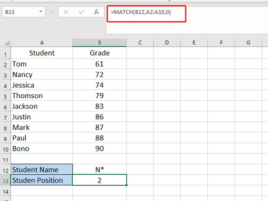
If we need to know the student position of N*, we can enter =MATCH(B12,A2:A10,0) in cell B13. So we know the second one is Nancy.

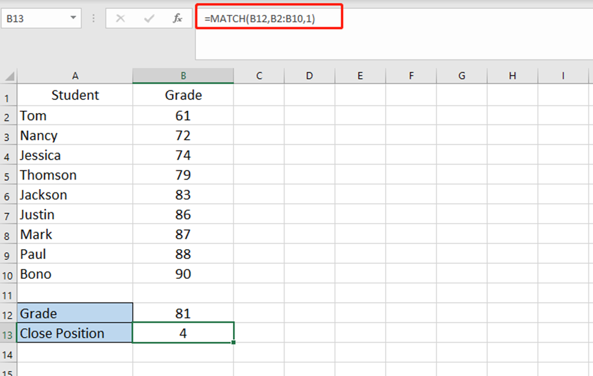
If we want to get the grade most close to 81 in the list, we can enter =MATCH(B12,B2:B10,1) in cell B13. Now we know Thomson’s grade is the one which most close to 81.