Microsoft Excel doesn’t wrap text by default, no matter how much text you enter in one cell. This could lead to the content of cells beside being covered, and finally affect the layout of the entire Excel spreadsheet. To avoid this , you can try these methods to wrap text in Microsoft Excel manually or automatically.
In general, you can use the Wrap Text feature in Home tab of Excel so that the contents will be self-adapting, which means it will fit the column width and be wrapped automatically. But if you only want to make changes to a few cells, or have some specific requirements, you can also use the shortcuts [Alt+Enter] to wrap text in Excel manually. It won’t fit the column width automatically but enables you to customize the location to wrap lines.
Wrap Text in Excel Automatically
1. Select all the cells you want to make changes, and go to Home tab.
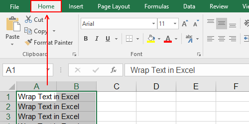
2. Click Wrap Text in Alignment section.
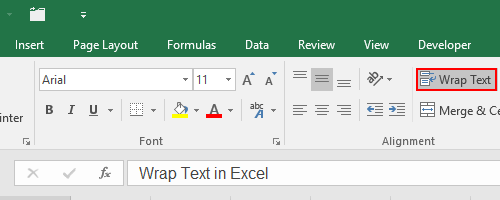
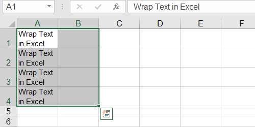
3. Thus the text in selected cells will be wrapped automatically.
Wrap Text in Excel Manually
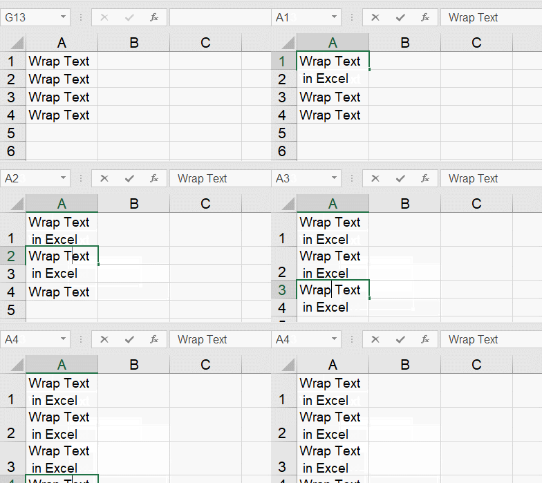
1. Place the cursor at the place you want to wrap the text and press [Alt+Enter].
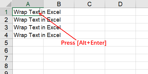
2. The text after the cursor will be assigned to the next line in the cell.
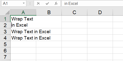
Using Find and Replace to Wrap Text in Batch
1. In addition to above methods, you can also wrap text using Find and Replace. But before that you must add some symbols as the separator between the text of two lines, such as commas. Then select all the cells you want to wrap text.
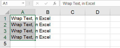
2. Press [Ctrl+H] to open the Find and Replace window. Enter “,” in Find what, and press [Ctrl+J] in Replace with.
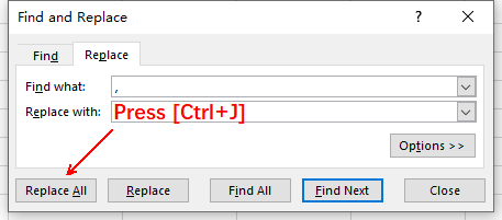
3. Hit Replace All and all the selected cells will be wrapped automatically. If you can’t see the text in the second line, just double click the cells to display the full content.

Thank you for the article.